Modelling of Grover's quantum search algorithms: implementations of simple quantum simulators on classical computers

Author: Ulyanov Sergey, Reshetnikov Andrey, Tyatyushkina Olga
Journal: Сетевое научное издание «Системный анализ в науке и образовании» @journal-sanse
Article in issue: 3, 2020.
Free access
Models of Grover’s search algorithm is reviewed to build the foundation for the other algorithms. Thereafter, some preliminary modifications of the original algorithms by others are stated, that increases the applicability of the search procedure. A general quantum computation on an isolated system can be represented by a unitary matrix. In order to execute such a computation on a quantum computer, it is common to decompose the unitary into a quantum circuit, i.e., a sequence of quantum gates that can be physically implemented on a given architecture. There are different universal gate sets for quantum computation. Here we choose the universal gate set consisting of CNOT and single-qubit gates. We measure the cost of a circuit by the number of CNOT gates as they are usually more difficult to implement than single qubit gates and since the number of single-qubit gates is bounded by about twice the number of CNOT’s.
Quantum computation, grover's search algorithm, quantum search algorithm's models
Short address: https://sciup.org/14123320
IDR: 14123320 | UDC: 512.6,
Моделирование алгоритмов квантового поиска Гровера: реализация простых квантовых симуляторов на классических компьютерах
В данной статье рассматриваются модели алгоритма поиска Гровера, служащего основой для разработки моделей других поисковых алгоритмов. Приведены некоторые модификации исходных алгоритмов, что расширяет возможности применения процедуры поиска. Квантовые вычисления в изолированной системе могут быть представлены унитарной матрицей. Чтобы выполнить такое вычисление на квантовом компьютере, обычно разлагают унитарную систему на квантовую схему, то есть последовательность квантовых логических вентилей, которые могут быть физически реализованы на данной архитектуре. Существуют различные универсальные наборы вентилей для квантовых вычислений. В статье описан универсальный набор вентилей, состоящий из CNOT и однокубитовых вентилей. Сложность схемы определяется по количеству вентилей CNOT, поскольку их обычно сложнее реализовать, чем вентили с одним кубитом, поскольку количество вентилей с одним кубитом ограничено примерно вдвое большим количеством вентилей CNOT.
Text of the scientific article Modelling of Grover's quantum search algorithms: implementations of simple quantum simulators on classical computers
In 1996 L. Grover devised an algorithm to search an unsorted database quadratically faster than any known classical algorithm can achieve. A common analogy for this algorithm is to search through a phone book for a person’s name knowing only their phone number. Without having the person’s name, the phone book becomes an unsorted database and a classical search could become very tedious. On average, one would have to make N queries, where N is the number of the entries in the phone book. However, if the correlation between the name and the phone number is encoded with quantum bits, the search is reduced to approximately N queries instead of N/2 as in classical search. The field of quantum algorithm development came into focus in the mid-1980s with the works of David Deutsch and others.
A decade later, Peter Shor showed an advantage of quantum computing over classical computation in practical disciplines like cryptography leading to widespread research boost in this domain. Shor’s algorithm for factorization (see Appendix 1) is often partnered with Grover’s search algorithm as the two most popular quantum algorithms for demonstrating practical computational advantage. Many quantum algorithms have been developed since then. A curated directory can be found in the Quantum Algorithm Zoo, which categorically describes the various quantum algorithm. The first category is Algebraic Number Theoretic. It includes problems like factoring, discrete-log, Pell’s equation, verifying matrix products, constraint satisfaction, etc. The Approximation and Simulation category includes problems like quantum simulation, adiabatic algorithms, semi-definite programming, Zeta functions, simulated annealing, etc. However, the category that interests this thesis most are the Oracular algorithms. This includes many sub-categories like searching, Abelian Hidden Subgroup, non-Abelian Hidden Subgroup, Bernstein-Vazirani, Deutsch-Jozsa, structured search, pattern matching, welded tree, graph collision, matrix commutativity, counterfeit coins, search with wildcards, network flows, machine learning, and many more. Note, not all these algorithms provide a superpolynomial speedup. New fields of quantum algorithms research employ applying the rules of quantum mechanics to game theory to model the situation of conflict between competing agents. The impact of quantum information processing on classical scenarios can be studied. Quantum games can be also used to analyses typical quantum situations like state estimation and cloning. Quantum walks also provide another promising method for developing new quantum algorithms. It was also shown that quantum walks can be used to perform a universal quantum computation. The development of quantum algorithms is a very lively area of research. However, the focus is on a small part of this landscape.
The core of the quantum algorithm is modeled as a kernel that would allow indexing a search string in the reference string. Since no pre-processing is done on the reference string, except slicing it to the search string size chunks, the database is essentially unsorted. L. Grover describes the quantum approach to solving the search problem in such an unstructured database. A closer look at Grover’s search is elucidated here. It is the foundation for the more specialized algorithms. In the original Grover’s algorithm, there is exactly one item which matches the search criteria. The artificial mathematical formalism of Grover’s search is to reduce the number of queries required to the database to find the answer by a polynomial (more specifically, quadratic) factor. A one-to-one correlation between the classical worst-case time of 0(N~) queries (N being equal to the number of database entries), and the quantum run-time of 0(^N) is not fully justified, as the quantum query itself works in a different technique, evolving the entire superposition of the database states. However, this is the inherent parallelism of quantum algorithms that we tend to harness. Zalka (1999) shown that Grover search is however provably optimal, thus no other algorithm, classical or quantum, can give a better runtime with the same initial conditions. However, it makes up for the lower (with respect to QFT) speed-up benefit in two ways: 1) Grover assumes an unstructured database search, which is rarely the case. We often have some idea of the data which can be exploited; 2) Searching is a very general problem in computer science and thus the impact factor of the time reduction is of great interest to researchers.
Models of quantum search algorithms
An alternate view of Grover’s algorithm can be” inverting a function” instead of” searching a database”. Given a function у = /(%) that can be evaluated on a quantum computer, Grover’s algorithm can calculate %. It can be used to efficiently determine the number of solutions to an N-item search problem, allowing it to perform exhaustive searches on solutions of NP-complete problems, reducing the required computational resource (see, Fig. 1).
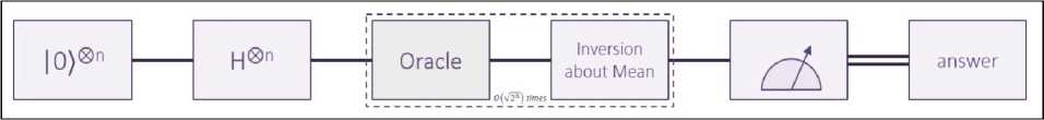
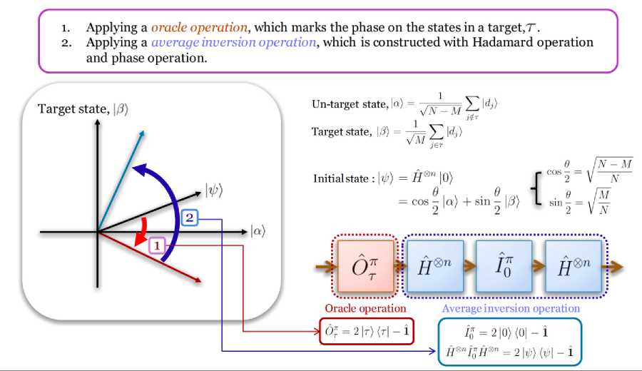
Fig. 1. Grover search steps and geometric interpretation of oracle and inversion operations
Grover’s search starts out with an equal superposition of states, i.e. each database entry has an equal
| N -1
probability of being the answer. The initial state can be described as: | ^ 0) = —;= ^| i ) . It is an oracular V N 1 =0
algorithm, i.e. it assumes the existence of an Oracle function (a common algorithm construct), which can produce an “yes” or “no” answer for a query in constant time. In the search procedure, the Oracle is consulted, which rotates the phase of the answer by я radians. Thus, the Unitary matrix is a diagonal matrix with all diagonal elements being 1 except at the row/column where the search entry and can be described as:
f 0,
if / * k
I ^ 1) = O ^ o),
Ojk = 1-W * k and / = i
1, otherwise
The next step is an inversion about the mean value of the states. This is known as the Grover gate, or the diffusion operator which is responsible for the amplitude amplification of the result. This operation can be described as: | ^2 = g G | ^ }, G = 21 ^)lyx | - 1 (the prototype of the Householder reflection).
Remark . Let Ц be a state on n qubits. We say that a unitary state preparation ( SP v ) on n qubits implements state preparation for Ц if SPs |0) = Ц . We start by presenting a useful pivoting algorithm for permuting entries in a sparse state such that all nonzero entries are grouped together. The idea is to then perform a decomposition scheme for dense state preparation on the grouped entries, which correspond to the state of a subset of the n qubits. Although several decompositions are known for general isometries, here we focus on a method based on Householder reflections that adapts well in the case of sparse isometries. We consider the task of breaking down a quantum computation given as an isometry into C-nots and single-qubit gates, while keeping the number of C-not gates small.
Generalized Householder reflections. Given a unit vector 1|, the standard Householder reflection with respect to 1| is defined as H9 = I — Ц Ц . We call 1| the Householder vector associated with the reflection. The generalized Householder reflection of phase ф with respect to Ц is defined as Hф = I + (eiu -1)|H|. and coincides with the standard definition if ф = n. On certain architectures generalized Householder reflections can be implemented directly and in a fault tolerant way. Standard Householder reflections can be approximated well using Clifford and T gates. In the circuit model a state preparation scheme can be used to perform a generalized Householder reflection. Let SPv denote a unitary implementing state preparation for the state 1| and Hф the Householder reflection with respect to 10) . Then Hф = Sp • Hф • SP9". Given two states 1| and | w^ we can construct a gate that maps 1| to e6 | w । t 1| - ei61 w\ for some real 6 using a standard Householder reflection defined as Hlw = Hu, where | u) = й-—, with 6 = n - arg (I | w) or 6 = 0 if I | w^ = 0. We also define the generalized Householder reflection
H».. = H, |u>=
1| -1 w III1 -I wll
e = | w - 1
1 - Ц w)
which has the property H w Ц = | w ). Householder reflections provide a straightforward method for implementing arbitrary isometries. Let Ц = V 10) be the first column of V and consider H^ 0, the Householder reflection mapping | 0) to |0) up to a phase. We can reduce the first column (and row by orthogonality) of V by applying the Householder reflection to the isometry, i.e., the only entry in the first row and column of HV is that corresponding to 00. Using the same idea, the isometry can be reduced column by column to a diagonal isometry. Applying a diagonal gate on m qubits then yields I n,m . For a schematic representation of the decomposition see as following
It is the basic idea of the Householder decomposition for dense isometries. Here * represents an arbitrary complex entry. Each step reduces one column without affecting the previous columns. The rows are reduced automatically due to the orthogonality of the columns. The final diagonal gate sets the phases on the diagonal equal to one. Let V be an isometry. Let | , .^ = V| j ) be the j th column of V and i be the target row index. For 5 ^ i and t ^ j we have
(i I H , V 1 t =M H ^ , i V I j =0, ( ‘ I H ^ , i V I j = e *
and
(s H V A = M V 1 + e~* ^ j
sV j iVt
1 +< i l V I »
Grover search guarantees the probability of the solution state to reach near unity on iterating the last two steps N times.
Brief review of quantum search algorithm’s models
Let us consider any particularities of Grover’s quantum search algorithm and its modification.
Grover’s Algorithm. The quantum oracle U f flips the ancillary qubit, if the target state t is fed in.
The ancillary qubit can be prepared in the superposition state H Ц = (| 0^ — 11) / sp2. Then the oracle gives a sign flip acting on the target state:
Uf (Iy ® H )| x) ® Ц = (—1)—f(x)(Iy ® H )| x) ® 11
For convenience, we denote the oracle Uf as Ut = I — 2| t)(t\ if the ancillary qubit H Ц is prepared.
The general phase flip can be constructed as follows: Ut ф = I^ n — ( 1 — e ф ) |Ц|. The generalized oracle
U has applications in the sure success search algorithm (see below) and the fixed point search algorithm
(for an unknown number of target states). Note that the operator Ut ффф ^ n ) can be realized by two quantum oracles U f . Having seen two defining attributes, the fixed-point property and optimality, of the success probability (see below), let us now create it using the operators provided: the state preparation A and oracle U . This problem simplifies when interpreted in the two-dimensional subspace Г spanned by M and T^
rather than in the full 2 n dimensional Hilbert space of all n qubits. First, define tt^ = e i T and
I t ) = (Is)— (tls)) / ^1— 1
so
that | s ^ = 11 — 1 1 1 ) + H 11 =
' 41—1'
V 1 7
. The matrix notation comes from
the definitions
I t) =
" 0 "V 1 7
and 1 1 ^ =
Г 1)V 0 j
The location of
s
on the Bloch sphere is in the XZ-plane at an
angle ф from the north pole, where ф G [0, n ] is defined by sin( ф /2) = ^k. We are given a unitary operator
A that prepares the initial state |s^ = A|0^ . From |s^, we would like to extract the target state TT^ with success probability Pl >1-52, where the overlap (T|s^ = V1e‘^ is not zero and 5 G [0,1] is given. To do so, it is provided with the oracle U which flips an ancilla qubit when fed the target state. That is, {7|T^|^ = T|6 ® 1 and ^|Г^|^ = 1^)1^) for TT T^ = 0. Below, it is shown how to solve this problem and extract T by performing on s a quantum circuit consisting of A, A†, U, and efficiently implementable n-qubit gates, such that
V. = 1 Tl^k) I2 = 1 - ST (T^ (1/5) VT! )2 .
Here T L ( x ) = cos( L cos -1 ( x )) is the L th Chebyshev polynomial of the first kind and L -1 is the query complexity: the number of times U is applied in the circuit . Furthermore, It is possible (see Fig. 2 below) construct for any odd integer L ≥ 1 and any δ .
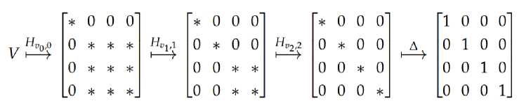
Some examples of P L and a comparison to the π /3-algorithm are shown in Fig. 2.
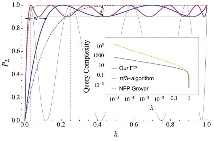
Fig. 2. A comparison of search algorithms, plotting the overlap P L of the target state with the output state versus the overlap λ of the target state with the initial state
[The fixed-point (FP) algorithm (thick solid) weigh against the π/3-algorithm (dashed) for the task of achieving output success probability P L greater than 1 - δ2 = 0.9 for all λ > λ 0 . The query complexity of the algorithms varies based on λ 0 (dotted vertical lines). For λ 0 = 0.25 (blue), the algorithm makes 4 queries while the π/3-algorithm makes 8. For λ 0 = 0.03 (red), the algorithm makes 12 queries while the π/3-algorithm makes 80. For comparison, also shown is Grover’s non-fixed-point (NFP) search with 8 queries (thin black). The width and error for the 4-query algorithm are labeled w and δ, respectively. (Inset) the query complexity is ploted against λ for the algorithm with δ2 = 0.1 (solid), the π/3-algorithm (dashed), and non-fixed-point
Grover’s (dotted). While the FP-algorithm and Grover’s NFP algorithm scale as L ∼ 1/√λ, the π/3-algorithm scales as L ∼ 1/λ]
Similarly, Grover’s reflection operators can be interpreted as SU (2) unitaries acting on Г . Arbitrary phases added to the reflections to define generalized reflections.
In Fig. 3 we show explicitly how to implement these generalized reflections using A , U , and efficiently implementable n -qubit operations.
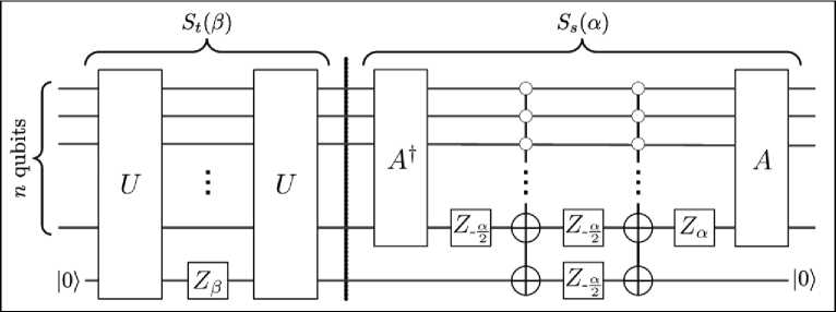
Fig. 3. A circuit for performing the generalized Grover iterate G(α, β) up to a global phase
[Here, Z θ := R 0 (θ) represents a rotation about the z-axis by angle θ. The first part of the circuit, before the dotted line, performs e-iβ/2St(β) and the second part performs S s (α). One ancilla bit initialized as 0 is required for both parts, but can be reused. The multiply-controlled NOT gates in the S s (α) circuit do not pose a substantial overhead – they can be implemented with O(n2) single qubit and CNOT gates or O(n) such gates and O(n) ancillas]
Their SU (2) representations are:
S s ( a ) = I - (1 - e- " )| s )M
S t ( в ) = 1 - ( 1 - ee * )| t)( t |-[ 1
1 - (1 - e ш) Я - (1 - e ш) V ЯЯ- (1 - e ш) V ЯЯ 1 - (1 - e a) Я
e e
where λ = 1 - λ. The product of the reflection operators is often
called the Grover iterate G (α, β) = - S s (α) S t (β). The original Grover iterate used α = ±π and β = ±π. The generalized reflection operators are also expressible as rotations on the Bloch sphere. Defining
R V ( 6 ) = exp
^- i ^0 (cos (v ) Z
+ sin ( V ) X ) I for Pauli operators X and Z , it
is find that
S, (a) = r-"2R, (a), St (в) = r'e/2R, (в)
When α = ±π and β = ±π, these rotations map the XZ-plane to the XZ-plane, reproducing the O(1) rotation picture of Grover’s original non-fixed-point (NFP)-algorithm.
The goal of achieving the PL is equivalently expressed as constructing, up to a global phase, the Cheby- shev state
I Cl) = Я-РТ I' ) + PLe^' 10 =
Я- P V P"etr
for some relative phase χ. For large enough λ, the
Chebyshev state lies near the south pole of the Bloch sphere.
An example run for the search is shown in Fig. 4.
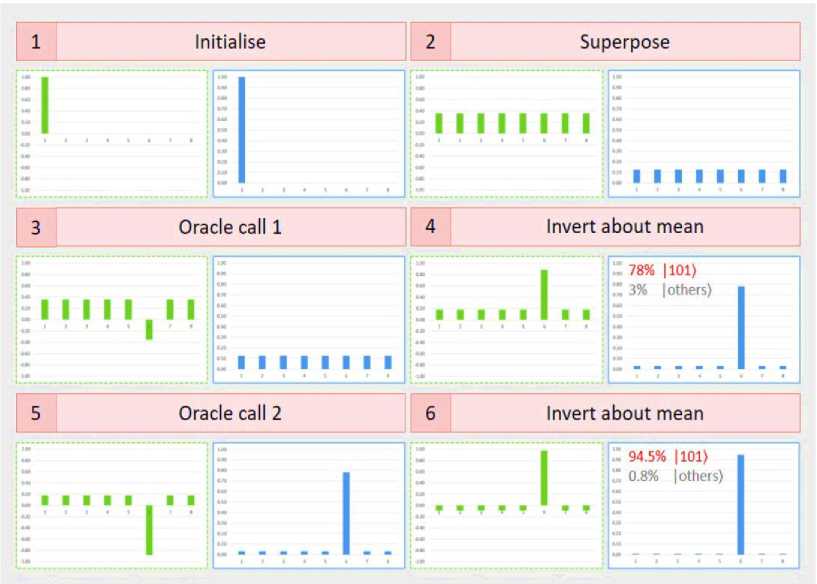
Fig. 4. Grover search example for 3 qubits
For the 3-qubit case, there are a total of 6 steps as the iteration requirement is 223 « 2 for the Oracle and inversion about mean step. At each step, the internal real amplitude of the states is shown in green (left), and its squared value, the measurement probability is shown in blue (right). The initialization step erases each qubit’s state, resetting it to |0). Then, the Hadamard gate on each qubit takes the state to an equal superposition of every possible 3-qubit basis states (3-bit binary strings). The next step is the Oracle call, which is a black box for the algorithm. It marks one of the states by inverting it (rotating it by я). However, this negative sign has no effect on the measurement probability. The amplitude is amplified by the inversion about mean step. The first run gives a measurement probability of 78%. Repeating it for the optimal number of iterations increases it to 94.5%.
For a detailed algebraic analysis, let the state at iteration j of the Grover search be:
| у ( k j , l j )^ = k j | i 0) + ^ l j 1 i) , where k ( i # i о
= l0 =
The first step of the iteration marks i 0, to flip the state to — k^ | i 0 ^. The mean is thus given by:
М 3
N
Each state gets transformed by the Grover gate from a | i ) to ( 2 ^. — a ) | i )•
Thus, the recursive relation for the states can be expressed as:
k v + i
2 ( N — 1) Ц— ^
N
— (— kj) =
N
j
N
j
,
(N
— 1)
l,
—
k, , x
(
—
2
)
k
+
(
N
—
2
)
i
N
j
N
j
l
j
+
1
(---j — L — k. =
N
jj
The recurrence can be solved by taking
1/
N
=
sin2
0
, to give the closed-form equation:
kj
=
sin
(
2
j
+
1
)
0
and
lj
= ^
cos
(
2
j
+
1
)
0
.
Setting k2 = 1, where jopt is the optimal number of iterations, we get, jopt
(
2
m
+
1
)
п
-
2
0
_ (
2
m
+
1
)
п
-
2sin
—
1
(
1/
4N
)
4
0
4 sin
-
1
(
1/ V
N
)
where
m
e Z
However, the equation is continuous while
j
e Z+
.
Approximating the equation, if we iterate
^
п
^^ /4
N
is large.
times, the probability of failure is just 1 /
N
when
Generalizing quantum search algorithms Grover’s search was enhanced by two subsequent research that will allow us to apply this search in the context. The improvements discussed in this section are:
- Multiple known number of solutions;
- Arbitrary distribution of initial amplitude;
- Multiple unknown number of solutions by randomizing iterations over multiple runs;
- Multiple unknown number of solutions by counting number of solutions.
Multiple known solutions. The case for multiple known solutions is considered first. Let t be the num- ber of solutions (known in advance), and S be the set of states considered as solutions. The transformation generalizes to:
I
v
(
k
j
,
lj^
=
Z
k
j№
+
Z
lj№ i
e
S i
e
S
V
N
-
2
t,
2 (
N
-
t
),
-
2
t,
------kf
+ -^-----
2 l
,.,—
к,
+
N
j
N
j
N
j
N
- 2
t
N
= |
v
(
k
j
+
1
,
l
j
+
i
))
The modification involves taking
t
/
N
=
sin
2
0
, to give the solutions as:
kj
= -^
sin
(
2
j
+
1
)
0
and
l}
=
N
-
t
cos
(
2
j
+
1
)
0
The probability of measuring any one of the solution states is maximized when l is close to 0, which yields the relation:
j
opt
( 2 m +1) п - 20 ( 2 m + 1) п - 2sin-1 (t / VN)
4
0
4 sin
1
(
t
/ V
N
)
, where
m
e Z
which can now be approximated for integer iteration as
п
N
4
t
. The solution state probability upper-
bounded by 1 /
t
, can now be written wholly in terms of
t
and
N
as:
kopt
=
"sin
Arbitrary initial amplitude
.
The second improvement that is needed is to consider an arbitrary initial amplitude for multiple known solutions. Instead of working with the amplitudes directly, the mean and variance of the solution and non-solution states are considered.
kj =1Z kjand ^k =1Z lk - k|2; lj = тр- Z ljand ^i2=тр7 Z l- l"|2.
t
i
e
S
t
i
e
S
N
-
t
i
e
S
N
-
t
i
e
S
Note, the variance equations are time-independe
n
t. T
h
e mean over these states after the solution states
(N -1) Tj - tkj are marked (Oracle called) is given by: ц. =--------------. The dynamics dictated by Grover’s algorithm jN can be described by the time-dependence of this average, giving the recurrences as: k^T = 2ц. + kj and lj+1 = 2^. — lj. Since the 2/7j factors are added to every term in the set, the mean itself evolves as:
kj+
, =
2
^
+
kj
and
lj+
t =
2
^
—
lj
. The solution to this recursion in closed-from is given by:
k
=
k
0
cos
(
m
j
)
+
1
0
N
—
t
t
sin
(
m
j
)
,
and
lj
=
l
0 cos
(
m
j
)
-
k0
t
N
-
1
sin
(
m
j
)
.
where,
m
=
cos
i
(
1
-
2L
I
N
. The optimal number of iterations and probability of success is given by:
n
k
)
. m
+
1)--2tan 1 ------
' 2
I
l
o\
N
-
1
J
P
max
=
1
-
2 |
l
-
l
| .
i
£
S
~ -1
(
1 2
1
^
2 cos 1 I NJ
These two relations are very useful as
j
is used to calculate the number of iterations that the program needs, and thereby the number of gates that would be executed. The
P
value helps in understanding the applicability of the search algorithm on a given set of data.
Multiple unknown solutions (by randomizing iterations of multiple runs. The next modification that is needed is the case for multiple solutions when the number of solutions is not known in advance. There are two ways in which such a problem can be attacked. When the number of solutions is not known, the number of required iterations cannot be predicted in advance. Thus, if a random iteration limit is chosen over all possible values for iterations (from the value for 1 solution to all states being solution states), then with a finite probability, the right number of iterations will be chosen. If this probability is high, the solution state is amplified with a high probability. This is the intuition behind the first method. Using trigonometric formula for compound angles and summation trigonometric series expansions, for real numbers а, в and an arbi trary positive integer 5, we can derive:
5
-
1
2 cos (a + 2pj ) = j=o sin (5p) cos (a + (5 -1) в)
sin
(
в
)
for the case,
E
5
-1 z
x sin
(
2
5a
)
cos
(
(
2
j
+
1
)
a
) = —------
.
j
=0 x ' 2 sin
a
Let t be the number of unknown solutions. The total probability of measuring a solution state after j iteration (using previously derived relations and |S| = 1 ) is, Psoh = 2k2 = sin"! ((2 j +1)6) . The average i e S success probability when 0 < j < 5 (and simplified by the relation 2 sin2 у = 1 - cos (2/), is, P5 = 12 sin
5
-
1 1
1
5
-
1
(2 j +1)6 = — 2(1 - cos (2 (2, j +1)6))
2
5
j
=
0
1 sin
(
4
56
)
2
-
4
5
sin
(
2
6
)
.
To get a
P
more than 1/4, the second term should be less than 1/4. Since can be chosen as,
11 1N sin (26) • L • -1 ) ? [ 7 2J(N -1) 1 ‘ sin 2sin . — 2. —, 1/ ( NN J VnV n Thus, the value to be chosen for 5, and thus the number of iterations to be performed, depends on the fraction of states that are solution. Now for the algorithm, an arbitrary value of 5 is chosen, and another increment factor 1 < A < 4/3 is chosen. At each iteration, the Grover’s search is performed with 0 < j < 5 If the measurement result after j iteration is not the solution, 5 is incremented to min (X5, 'JN). The value of 5 on the rth such iteration is Ar - 15. Let 5C = 1/sin (26). The critical stage is reached when rc =Tlog ^5c 1 .
This happens with probability,
1
(
1
-
P,,-
)=1I
1
-
1
+
sin
(
^x
’ r
=
1
(
2
45
sin
(
2
0
)
. The expected number of it-
eration when the critical state is reached (if at all it reaches, observed
P
for rounds before it is 1), is thus expanded (using geometric series expansion),
_ 1 ^Я
'
-5!
—0 <
5
(
1
1"”
‘c-
0
<
5
(
15
c
-1)
<
515
,
E
I
Г
I
51
— — <
.
L cJ
2 £ 2
(
1
-
1
)
2
(
1
-
1
)
2
(
1
-
1
)
2
(
1
-
1
)
After the critical stage, further increase in
5
always succeeds with probability greater than 1/4. Thus, the limiting case is reached when
Pfai
z =
3/4
and is upper bounded by,
^
J
r
,
^
uv Г
E
[
r
]
=
1
VI
3
I
1
1
u
+
r
,
=
1
VI
3
1
I =
1
L
c
1
2
11
4
J
4 8
11
4
J
8
T^
I
1--
4
J
1
Flog
A
"1
8
-
6
1
. The total expected number of iteration of the Grover algorithm (each time with different number of
Grover iterations in them), when
t <
3
N
/4,
5
= 1 and Л = 6/5 can be derived as
51^ 53c 4
3
V
9
N J N
I
E
I
r
1
+
E\r+
l< ——— +--— =
3
+ —
5
=—, =
O . —
.
I
c
J
L
^
J
2
(
1
-
1
)
8
-
6
1
(
2
J
c
4.
(
N
-
t
)
t
П
t
This is approximately 4 times the number of iterations had
t
been known in advance. The case for no solution is handled with a time-out, while the case for
t
> 3/4 can be solved in constant time by classical sampling.
Multiple unknown solutions (by counting). The second method for multiple solutions is more intuitive. It divides the algorithm into two steps. In the first step, another quantum algorithm counts the number of solutions and then, the algorithm for known multiple solution is used to maximize the solution probability. Formally, counting is the cardinality of an inverse Boolean function В with input 1: t = |B-1 (1)|. There are different ways to do quantum counting. The first method is by using quantum Fourier transform (QFT) to find the period 6 as kj evolves, to find t. The number of iterations executed is encoded as part of the state, I V 2y -1Г 1 (A
I
V
(
k„
l
,
,
Y
Ы
41
ID
1
1
,
1
-
) +
1
l
,
l
-)
j=0 L \2Y V -eS -vSJ Now, if the original qubits in | i) is observed, the state collapses to (within normalization factors), 2Y -12 1 kj | -^ or 1 lj | -^ . Running discreet QFT on this state, on measurement, with high probability the value f j=o can be estimated. The number of solutions can be calculated as, t = sin2 (f n /2Y) The value of / helps to balance the accuracy with run-time and needs to be typically increased gradually over multiple runs until f becomes large. Another conceptually simpler way to count is to determine the fraction of state marked by the Oracle. A state is created such that an extra qubit is 11) if it is a solution, |0) otherwise, IV(k,,l )) = 1 k,|/)|1)+1 lj\-l|0).
-
e
S -
v
s
Now, measurement by state tomographic trials on this qubit gives the proportion of solution state to the total number of states with increasing degree of accuracy. An arbitrary amplitude and multiple solutions without counting is based on finding the number of times the original Grover algorithm is to be run. However, quantum counting involves states and procedures that are different from the qubit encoding of Grover. The second method is decomposed to the required Oracle unitary. Let the Oracle is based on the Boolean function , such that it’s elements, bi е{0,1}, i g{0" •( N -1)} is marked when it is a solution state. The unitary matrix is formed such that the most-significant qubit is the count qubit. In terms of diagonal matrices and element-wise subtraction it can be written as, Ocount
diag
(
1
-
В)
diag
(-B)
diag (-B) diag (1 - B)
Remark
. Grover’s algorithm (or the variants discussed in the previous section) cannot be directly used for pattern matching. In Grover’s search, the initial input state is an equal superposition of all the possible strings of the size of the search pattern. Thus, the number of states in the superposition is
AM
. The Oracle then marks the answer state so that the output is the search pattern. However, if the index of the pattern matching is the requirement, the state needs to be initialized such that it stores a superposition of indices in
N
–
M
+ 1. The Oracle marks the index where the pattern matches. So, in a naive Grover’s search implementation, the entire pattern matching comparison is off-loaded to the Oracle, and the algorithm is not useful without a description of the Oracle construction. The Oracle, however, is a unitary matrix with the diagonal elements being – 1 for the answer index and 1 otherwise. Thus, the
answer needs to be known for the Oracle construction
, the exact problem that needs to be avoided to practically program a pattern matching application.
For matching a sub-string, only a sequential set needs to be considered.
In Grover’s search, the Oracle function basically stores the relationship between the database and the search string. This relationship thus needs to change for each search string, making it impractical for implementation. The key idea in quantum pattern matching is to define a “compile once, run many” approach for the Oracle.
The algorithm defines multiple Oracles, one for each character of the alphabet.
The Boolean function that the Oracle encodes is – 1 for the indices where the reference string matches the Oracle’s defining character
а E
E:
f
^
:
{
0,1
}
2
^
{
-
1,1
}
.
The Boolean function that maps to
{
0,1
}
is converted to
{
-
1,1
}
by a phase-kickback process of
(
-
1
)
f
a
(
i
)
for implementing the gate level circuit for the Oracle function.
The Oracle construction is independent of the search string
, giving this algorithm its usefulness. The Oracle circuit assembly, however, depends on the search pattern as shown in the algorithm anatomy in Fig. 5.
Fig. 5. Algorithm anatomy
At every iteration step, all the
A
Oracles exist in the circuit but only one of them is control activated by the step’s corresponding character of the search pattern. Since the model of quantum computer is based on in-memory computation, the exact circuit need not be pre-compiled if the underlying micro-architecture and classical control are fast enough to allow real-time circuit interpretation.
The circuit for constructing an arbitrary Boolean function is not provided. The circuit is devised that allows generating an Oracle automatically in a high-level programming language in the kernel. In the implementation, a sequential run through the Boolean function is performed. If the state of a particular index needs to be marked, the Boolean value of the index is taken and a CPhase gate is applied on all the qubits to the Oracle, with inverted control on qubits where the Boolean index encoding is 0. Continuing the example, the
Boolean function for
Ci
acting on
q
‘ =
4
qubits is
f.
= [1, 1, 1, 0, 0, 0, 0, 0, 0, 0, 0, 0, 0, 0, 0, 0]. Thus, the positions of 0, 1, 2, or the qubit states of 10000), 10001), 10010) are marked using 3 CPhase Gates over 4 qubits. The first CPhase will have all the controls inverted, for the second CPhase
q
′
,
q
′
,
q
′
are inverted and for the third CPhase
q
′
,
q
′
,
q
′
are inverted. The inversion is carried out by wrapping Pauli-X gate on those qubits before and after the CPhase. The multi-qubit CPhase is converted to a multi-qubit CNOT by wrapping a Hadamard on one of the qubits and then decomposing. he third part of the circuit is the Grover amplification process over the entire non-ancilla qubit set. In the initialization circuit, the Oracle as well as for the Grover gate, the circuit construction uses
n
-qubit Controlled-X gates. These need to be decomposed to Toffoli using ancillas for the purpose of simulating.
The protocol for the algorithm is outlined in Fig. 6 for
n
qubits.
Fig. 6. Schematic diagram of Grover’s quantum search algorithm over a space of n qubits (N = 2n). An example of the distributions of quantum amplitudes at each stage are depicted at the right. Inversion about the mean. (a) Initially all of the database elements start in an equal super-position and the mean line (dotted line) lies in the middle of the distribution. (b) Flipping the amplitude of one of the marked states shifts the mean line of the distribution down. (c) When the whole distribution is inverted about this mean line, the amplitude of the marked state gets larger while the amplitude of the other states decreases. (d) After this process is repeated for a set number of times the probability of measuring the marked state becomes much greater than any of the other database elements
After initializing the system to the
0
⊗
n
state a Hadamard gate is applied to put all the states in an equal superposition. This assures that the algorithm starts with each database entry being equally likely, as shown on the right-hand side of Fig A2.4(a). The next step is the heart of the algorithm known as the “oracle query”, it quickly checks if a proposed input “
x”
is a solution to the search problem. Quantum mechanically this step is a mathematical function that marks a particular state of a quantum superposition by flipping the sign of its amplitude as shown in Fig. A2.4b). Following the oracle, a number of quantum operations amplify the weighting of the marked state independent of which state is marked (see Fig. A2.1). After many iterations of this query / amplification process, the marked state accumulates nearly all of the weight and is revealed following a measurement.
The required number of queries can be shown to be the integer closest to [
π /
(4sin
-
1
(
N-
1
/
2
))
-
1
/
2]. For
N =
1, the marked element would thus appear with high probability after approximately
π √N/
4 iterations, and for the special case of
N
= 4 elements, a single query would provide the marked element with unit probability.
Classically, a single query of a 4-element search space followed by a guess can only result in a successful outcome with 50% probability. In the following we will track the states of two qubits as each step of the algorithm is performed. First each qubit is initialized to the
0
state and the state of the system is written
0 0
. This is similar to initializing a classical register. Next a Hadamard gate is applied to each qubit. This operation performs the transformation |0^
^ 10^ +
Ц
. Directly following the Hadamard gate the state of the two-qubit system is
A, [(I o)+|1))®(| o)+|1) )]=-t □ 0>|0>+| O>|1>+Цо)+Ц ]. This puts all of the database elements in an equal superposition.
Next the oracle query is performed. This step takes some state
x
and adds a minus sign to the amplitude giving
— |
x
^.
The oracle will be explained in more detail later. For now, it is just a mathematical function that flips the phase of one of the database elements by 180
◦
. For this example, the state
01
will be marked (i.e. the amplitude of this state will be inverted), but in theory any of the four states could be marked. The state now becomes
^^[l0)|0)-10)Ц + Ц|0) + Ц]
• The next three operations in Fig. A2.1 perform a state amplification process. Here the amplitude of the marked state increases while the amplitude of the unmarked states decreases. The state amplification process is carried out by performing an inversion about the mean, as shown in Fig. A2.1.b. Here the amplitude of the marked state increases while the amplitude of the unmarked states decreases. The state amplification process is carried out by performing an inversion about the mean, as shown in Fig. A2.1. Since the marked state has an amplitude that is 180
◦
out of phase with the other elements in the database, the average of the four amplitudes is slightly below the mid-point of the three positive states. When the whole distribution is inverted about the mean, the marked state grows in amplitude while the unmarked states decrease in amplitude. For the example shown here the state after the amplification process is
( 010^ 10^ + 1|0^Ц + 0|Ц0^ + 0|Ц)
. All of the population is transferred into the marked state and the probability of finding the amplitude in any of the other three states goes to zero. This is a special case of Grover’s algorithm where after a single cycle of the algorithm, the marked state can be found with 100% probability. For other cases of the algorithm the cycle is repeated for a set number of times before the measurement occurs. As mentioned above the ideal number of times to repeat the protocol is the integer closest to [
π /
(4sin
-
1
(
N-
1
/
2
))
-
1
/
2]. If the sequence is repeated too many times then the amplitude of the marked state begins to decrease and the amplitude of the unmarked states begins to increase. As mentioned before the oracle query is the cornerstone of the algorithm. In the above explanation this step was treated as a mathematical function that marks one of the database elements. In the algorithm outlined by Grover this oracle query is a quantum database in and of itself. The oracle does not know the solution to a question in advance but can recognize the solution when it is inputted. This is done by a parallel bit wise search of all of the oracle’s database elements. When the oracle matches the input bit string with a bit string in its database then the amplitude of that state is inverted. The rest of the algorithm is carried out as explained above.
Example
:
Generalized Grover’s oracle and quantum partial search algorithm
. One query to oracle
U
t
combined with the diffusion operator
D
n
is called the Grover iteration or Grover operator:
Gn
=
DUt
. See Fig. 7a for the quantum circuit diagram of
Gn
.
Fig. 7. Quantum circuits of global Grover operator G
n
defined and local Grover operator.
[The diffusion operator D
n
(D
m
) is single-qubit-gate equivalent to the n-qubit Toffoli gate
Ли1 (
X
)
(m-qubit Toffoli gate Лт_х
(
X
)
. Here X and Z are Pauli gates, and H is the Hadamard gate. The subspace where D
m
acts can be chosen arbitrarily]
The diffusion operator
D
n
reflects the average of the whole database. The operator
G
n
is also called the global Grover iteration (global Grover operator). One Grover operator
G
n
uses one query to oracle
U
f
. Applying
G
n
iteratively on the initial state
s
, the amplitude of the target state will be amplified. After
j
Grover iterations, the success probability
P
n
(
j
) is
Pn (j ) = Itt I G I sn )Г = sin2 ((2j + 1) 9) , with sin 9 = 1/ 4N . When j reaches j^ = |_^VN / 4 J, the probability of finding the target state approaches 1. The maximal iteration number jmax is the square root of N. Clearly, Grover’s algorithm provides a quadratic speedup compared with the classical algorithm (in oracle complexity). The idea behind Grover’s algorithm can be generalized into the amplitude amplification algorithm. The success probability (finding the target state) does not scale linearly with the number of iterations. It suggests that Grover’s algorithm becomes less efficient when j approaches jmax. Previous works argued that the expected number of iterations j = Pn(j) has the minimum at jexp = ^0.583д/NJ, which is smaller than jmax. When j is jexp, the success probability is around 0.845. In practice, the iteration number jexp has a high probability to find the target state. The measurement result can be verified in classical ways. If the result fails, one has to run the algorithm again. The expected number of oracles is minimized at jexp. Quantum Partial Search Algorithm (QPSA). The QPSA was introduced by Grover and Radhakrishnan. Since Grover’s algorithm is optimal (in oracle complexity), the QPSA trades accuracy for speed. A database of N items is divided into K blocks: N = bK. Here b is the number of items in each block. It is assumed that the number b is also a power of 2: b = 2m. And the number of blocks is K = 2n – m. The QPSA can find the block which has the target state. In other words, the QPSA finds the partial (n – m)-bit of the target state (which is n bits long). The optimized QPSA can win over Grover’s algorithm a number scaling as b . A larger block size (less accuracy) gives a faster algorithm. Suppose that the address of the target state 1t^ is divided into |t^ = |t^®|t2). Here tx is (n — m) bits long and t2 is m bits long. The task is to find tx instead of the whole t. Besides the diffusion operator Dn, the QPSA introduces a new diffusion operator Dn,m: D„ =I I^—m Dn =I I in—m ®(2 smWm I — I-,m ) • The diffusion operator Dn, m reflects around the average in a n,m n,m m m block (simultaneously in each block). The diffusion operator Dn,m can be viewed as the rescaled version of Dn: the database with size 2n is rescaled into size 2m. It is possible define a new Grover operator as Gn m = Dn Ut, See Fig. 1b for the quantum circuit diagram of Gn,m. The diffusion operator Dn,m reflects the average of block items. The operator Gn,m is also called the local Grover iteration (local Grover operator). The QPSA requires a smaller number of oracles (the saved oracle number scales as b ) than Grover’s algorithm. Physical model implementation of quantum search algorithm
By implementing the search function as a quantum operator acting on a superposition, the Grover algorithm is able to somehow evaluate it in one single call for all possible input states. This so-called quantum parallelism provides the basis for the speed-up of the search in comparison to a classical algorithm. However, being able to encode the result of the search function in the phase of a multi-qubit state does not directly translate to a speed advantage since it is usually very hard to extract this phase information from the quantum state. Indeed, to extract the values of all phases from an
N
-qubit state, it would be necessary to perform
O
(2
N
) measurements on an ensemble of such identically prepared quantum states. However, extracting the amplitudes from such a state takes only
O
(
N
) measurements, that in addition can usually be carried out in parallel. It is for this reason that the Grover algorithm uses an operator that transforms the information encoded in the phases of the qubits to an information encoded in their amplitude. However, since the conversion between phase to amplitude information through the application of an unitary operator is limited by certain physical constraints, the algorithm needs to repeat the encode-and-transfer sequence described above
O
(√
N
) times. To analyze further the constraints and principles of the algorithm, we will discuss a more detailed derivation of it starting from the Schrödinger equation and we will also explain what limits the efficiency of the phase-to-amplitude conversion in the algorithm.
Deriving the Grover Algorithm from Schrödinger’s Equation An interesting derivation of the Grover algorithm starting from Schrödinger’s equation has been detailed by Grover himself and shall be briefly re-discussed here since it sheds light on the basic principles on which the algorithm is based. The derivation begins by considering a quantum system governed by Schrö-dinger’s equation, which can be written as (setting = 1 for better readability) . 5 z x a2 i — V ( x, t ) = - ^r V ( x, t) + V ( x ^¥ ( x, t) d t dx
Here
ψ
(
x
,
t
) describes the wave-function and
V
is a time-independent potential.
Let us assume that the potential
V
(
x
) is shaped as in Fig. 8, i.e. possessing a global minimum of energy.
Fig. 8. Wave function ψ(x) and potential V (x) defined on a grid of points x1, . . . , xN. [A minimum of the potential can encode a search value xi]
When one initializes the system to a state
ψ
0
(
x
,
t
0
) and lets it evolve for a given time,
ψ
(
x
,
t
) will be attracted by the minimum of potential energy and “fall into it” much like a classical particle in such a potential would. We might thus ask if we can encode the solution to a search problem as a point of minimum energy
x
0
of a potential
V
(
x
), take an initial state
ψ
0
(
x, t
0
) and let it evolve into a state that has a high probability around
x
0
, thereby solving the search problem.
To answer this question, it is first necessary to discretize the wave function
ψ
(
x, t
) such that it can represent the search problem stated in the last section, and which is defined over a finite number of states. In the simplest case, we can use a regular grid of points
x
i
with a spacing ∆
x
for this, as shown in Fig. A2.5.
Discretizing the time evolution in steps A
t
as well and defining
s
= A
t/Ax
2
. we obtain a new equation of
. , V'+A'
the form--
i—
—
t t , t
П
t
Vx
=
Vi
+X
+Vi
—X
—
2
Vx
A
t
A
x
2
—
V
(
x
)
v
t
, where we have written
у
(
X
i
, t
) =
y
*
. For a circular
grid with
N
points we can write this equation in matrix form as
V
+A
*
=
S
A
*
•
V
t
with
S
being a state transition matrix of the form
S =
1
—
2i
s —
iV
(
x
)
A
t i
s
i
s
1 — 2 is — iV ( x2 )A t isis ' •.
i
s
i
s
i
s
1
—
2i
s —
iV
(
xN
)
A
t
For infinitesimal times ∆
t
we can separate the effect of the potential
V
(
x
) on the wave function from the spatial dispersion a
i
s
by writing
S
A
t
-
D
•
R
with
(1 — 2 is D =
i
s
i
s
1
—
2
i
s
i
s
i
s
(
e
—
iV
(
x
1
)A
t
i
s
, R =
e
-iV
(
x
2
)A
*
0
e - iV
(
x
n
)
A
t
.
i
s
i
s
1
—
2i
s
This approximation is correct to order
O
(
s
)
up to an irrelevant renormalization factor.
Now, we can repeatedly apply the matrix product D·R to the wave function to obtain its state after a t / At A given finite time t by writing V0+t = П D • R V . This technique of splitting up the full evolution opera- tor into a product of two or more non-commuting operators that are applied repeatedly to the wave function to obtain its state after a finite time is sometimes referred to as Trotterization – in reference to the so-called Lie-Trotter formula on which it is based – and on which digital quantum simulation relies. The evolution of the wave function at infinitesimal times is governed by two processes: The interaction with the potential V and a diffusion process that mixes different spatial parts of the wave function with each other. The operator D resembles a Markov diffusion process since each row and column of the matrix sums up to unity, whereas R changes the phase of each element of the wave function as a function of the local potential seen by it. If we apply R to a fully superposed initial state of the form ψi = 1 (omitting the normalization factor for simplicity) and assume that Vi = 0 for i ^ j and VjAt = п/2 (the potential thus encoding a search function with C(j') = 1 and C(i) = 0 for i ^ j). the element у will get turned according to yj ^ i^j. whereas all other elements ψi will remain unchanged. Applying the operator D to the resulting state will transform ^ according to ^j ^ ^J(i + 2 s (1 + i)) with a corresponding amplitude ^1 + 4s + O (s2) and the adjacent states ψj±1 according to ψj±1 → ψj±1(1 -
s
(1 +
i
)) with an amplitude
^
1
—
2
s
+
O
(
s
2
)
. Hence there
is a transfer of amplitude between the state whose phase has been turned and its neighboring states.
If we reset the phases of all the
ψi
to zero afterwards, we can iterate the application of
D
·
R
until all of the amplitude has been transferred to the element
ψ
j
which corresponds to a solution to the search problem. This is, in essence, exactly what the Grover algorithm does, the only difference being that it replaces the matrix
D
with an unitary matrix that maximizes the amplitude transfer to the states solving the search problem, thereby speeding up the algorithm. As stated before, the efficiency with which the algorithm can transfer amplitude between different states is limited by physical constraints. In the next section, we will therefore discuss exactly what limits this efficiency and which unitary diffusion matrix one should choose to maximize it.
Remark. The unstructured search problem in constant time can be solve by computing with a physically motivated nonlinearity of the Gross–Pitaevskii type. This speedup comes, however, at the novel expense of increasing the time-measurement precision. Jointly optimizing these resource requirements results in an overall scaling of N1/4. This is a significant, but not unreasonable, improvement over the N1/2 scaling of Grover’s algorithm. Since the Gross–Pitaevskii equation approximates the multi-particle (linear) Schrodinger equation, for which Grover’s algorithm is optimal, the result leads to a quantum information-theoretic lower bound on the number of particles needed for this approximation to hold, asymptotically.
Efficiency of Quantum Searching.
As discussed by L. Grover, it is interesting to ask what is the maximum amount of amplitude that can be transferred in a single step of the Grover search algorithm and which matrix
D
should be chosen to maximize this transfer. To answer this question and derive the ideal diffusion matrix, we will assume first that, without loss of generality, the matrix
R
which encodes the value of the
N
-
1
search function C in the quantum state of the qubit register can be written as R = I — 2^ C (j )| j^ j| . This j=0
operator will flip the sign of all states for which
C
(
j
) = 1. Now, the next step consists in finding a diffusion or state transfer matrix which will maximize the amplitude transfer to states tagged by the Oracle operator above and which will also reset the phases of the quantum register to zero afterwards, such that we might apply the Oracle operator to the resulting state again. In the most general case, such a state transfer matrix will have the form
"
b a
a
a '
ab
a
a
D
c
=
V
a
a
b >
Here, we assume that all non-diagonal elements of the matrix are equal, which is well justified since we have no knowledge of the structure of the search space of the problem and therefore want to treat all basis states equally during the phase-to-amplitude conversion. Furthermore, since both the initial quantum state and the Oracle operator contain only real numbers and we demand that the quantum state after applying Dc may contain only positive real numbers as well it is easy to show that a, b must be real numbers. Finally, the unitarity of quantum operators demands that D£Dc = I, which for the matrix above is equivalent to the two conditions 1 = b2 + (N — 1) a2, 0 = 2ab + (N — 2) a2. Solving these two equations for a, b yields the trivial solution b = ±1, a = 0 and the more interesting one b = ± (1 - 2/N), a = ∓2/N. As can be checked easily, the solution b = 1 - 2/N, a = 2/N results in a maximum amplitude transfer from states i for which C(i) = 0 to states j for which C(j) = 1. Thus, the ideal diffusion matrix to be used in the Grover algorithm is given as
D
=
"—
1
+
2/
N
2/
N
2/
N
—
1
+
2/
N
2/
N
2/
N
• 2/
N '
• 2/
N
v
2/
N
2/
N
2/
N
• —
1
+
2/
N
,
This matrix, together with an Oracle operator
R
as given above will yield the maximum amplitude transfer from states not solving the search problem to states that solve it. Repeating the application of
D
·
R
on an initially fully superposed quantum state for
O
(√
N
) times will transform the input state to a state containing only the solutions of the search problem. For the two-qubit case, the Oracle and diffusion operators
R
and
D
of the previous sections are
'
(
—
1
)
C
(
00
)
0 0 0 '
"—
11 1 1
"
0
(
—
1
)
C
(
01
)
0 0
1
—
111
R
=
,
D
=
0 0
(
—
1
)
C
(
10
)
0
11
—
11
v
0 0 0
(
—
1
)
C
(
11)
v
v
1 1 1
—
L
Before discussing the experimental implementation of this algorithm, we will show how we can compare its computational efficiency to that of an equivalent classical algorithm in order to assess the achieved quantum speed-up.
Transition Probabilities in Generalized Quantum Search Hamiltonian Evolutions.
A relevant problem in quantum computing concerns how fast a source state can be driven into a target state according to Schrodinger’s quantum mechanical evolution specified by a suitable driving Hamiltonian. The computational aspects necessary to calculate the transition probability from a source state to a target state in a continuous time quantum search problem defined by a multi-parameter generalized time-independent Hamiltonian. In particular, quantifying the performance of a quantum search in terms of speed (minimum search time) and fidelity (maximum success probability), a variety of special cases that emerge from the generalized Hamiltonian. In the context of optimal quantum search considered, it is possible to outperform, in terms of minimum search time, the well-known Farhi-Gutmann analog quantum search algorithm find. In the context of nearly optimal quantum search, instead, it is possible to identify sub-optimal search algorithms capable of outperforming optimal search algorithms if only a sufficiently high success probability is sought. Finally, the relevance of a tradeoff between speed and fidelity with emphasis on issues of both theoretical and practical importance to quantum information processing discussed. Grover’s algorithm was presented in terms of a discrete sequence of unitary logic gates (digital quantum computation). Specifically, the transition probability from the source state |
^
^ to the target state |
y^
after the
k
-times sequential application of the so-called
Grover quantum def 2
vro„,
(
k
,
N
)
=
KI
Gk |^,>|
search iterate
=
sin
2
(
2
k
+
1
)
tan
1
Г 1 'v V N — 1 у G is given by,
In the limit of
N
approaching infinity,
P Grover approaches one if k = O (VN).
Remark
. We point out that the big
O
-notation
f
(
x
) =
O
(
g
(
x
)) means that there exist real constants
c
and
x
0
such that |
f
(
x
)| ≤
c
|
g
(
x
)| for any
x
≥
x
0
.
The temporal evolution of the state vector |
V
(
t
)^ of a closed quantum system is characterized by the Schrodinger equation,
ihdt | V
(
t
)^ = ?f (
t
)|
у
(
t
)^ . The Hamiltonian
14
(
t
)
encodes all relevant information about the time evolution of the quantum system. From a quantum computing standpoint, if the Hamiltonian
14
(
t
)
is known and properly designed, the quantum mechanical motion is known and the initial state (source state, |
^
) at
t
= 0 can potentially evolve to a given final state (target state, |
^
) at
t
=
T
. In particular, for any instant 0 <
t
<
T
, the probability T^ ^^ ^ that the system transitions from the state |
^
) to the state
|^)
under the working assumption of constant Hamiltonian is given by,
2
e
V
w
—
-Kt , h
—TYt . The unitary operator U = e h denotes the temporal evolu tion operator. Figure 9 displays a graphical depiction of the digital (discrete time) and analog (continuous time) quantum search algorithms. Fig. 9. Gate-level schematic of the (a) digital and (b) analog quantum search algorithms Grover’s quantum search algorithm provides a quadratic speedup over the classical one and the computational complexity is based on the number of queries to the oracle. However, depth is a more modern metric for noisy intermediate-scale quantum computers. Grover’s algorithm is not optimal in depth. A new depth optimization method for quantum search algorithms was proposed and a quantum search algorithm developed, which can be divided into several stages. Each stage has a new initialization, which is are scaling of the database. This decrease errors. The multistage design is natural for parallel running of the quantum search algorithm.
Remark
. Recently, more studies focused on the resource estimation, such as width and depth, for Grover’s algorithm instead of the traditional oracle complexity. Grover’s algorithm is optimal in oracle complexity. However, no research addressed the depth of the quantum search algorithm. Surprisingly, the depth of the diffusion operator can be reduced to one. However, these algorithms have (1/2) maximal successful probability, and the expected depth is not as efficient as the original Grover’s algorithm. Inspired by the quantum partial search algorithm (QPSA), a new depth optimization for the quantum search algorithm was introduced. The algorithm can have lower depth than Grover’s algorithm. To further lower the depth, a divide-and-conquer strategy (combined with depth optimization) can be applied. The divide-and-conquer strategy means that the search algorithm is realized by several stages. Each stage can find a partial address of the target state. The next-stage initial state is the rescaled version of the last-stage initial state. The divide-and-conquer strategy naturally allows the parallel running of the quantum search algorithm.
If the oracle takes much more depths than diffusion operator depth, then the oracle complexity will be approximately equivalent to the depth complexity. The ratio between oracle depth and diffusion operator depth was defined. Above a critical ratio, Grover’s algorithm is optimal in depth. Based on the depth optimization method the critical ratio defined as
O
(
n
-1
2
n
/2
). If the algorithm divided into two stages, the critical ratio is a constant.
Example
. Still shallow-depth algorithms can be realized on real quantum computers (for the noisy intermediate scale quantum (NISQ) era). The width (the number of physical qubits) represents the size of quantum computers. The algorithm’s depth (the number of consecutive gate operations) represents the physical implementation time for the algorithm. Multiplying the width and depth we get the quantum volume, which gives a metric for NISQ computers. Coherence time is limited in NISQ computers. A set of gates which can approximate any unitary operation is called the universal quantum gate set (Solovay - Kitaev theorem). It is assumeв that the quantum computer is equipped with a universal quantum gate set. So, the depth is counted by universal quantum gate operations. The quantum oracle
U
f
is realized by quantum gates from the universal quantum gate set. It is assumed that the depth of the quantum oracle scales polynomially with
n
. The oracle complexity would be equivalent to the depth complexity if the quantum oracle would be the only operation realized in Grover’s algorithm. However, it is not true. Another unitary operation (diffusion operator) is required for Grover’s algorithm. How to choose the diffusion operator is related to the initial state preparation. The unstructured population space
{
0,1
}
n
(database) can be prepared in an equal superposition state on a quantum computer polynomial efficiently:
\sn
=
h
H
°
n
|0)°
n
with single-qubit Hadamard gate
H
. Note that the initial state
s
can be efficiently prepared with a depth of one circuit. The diffusion operator has the constraint that the state
s
is the eigenvector of the diffusion operator with eigenvalue 1.
Working in a continuous time quantum computing framework, Farhi and Gutmann proposed an analog version of Grover's algorithm where the state of the quantum register evolves continuously in time under the action of a suitably chosen driving Hamiltonian (analog quantum computation). Specifically, the transition probability from the source state |
^
} to the target state |
^
^ after the application of the unitary continuous
-й FGtct time evolution operator UFG = e й for a closed quantum system described by a constant Hamiltonian
FG
is given by,
p Farhi-Gutmann def (k, N ) =
(Vw\e
K)
=
sin
2
Ex t h 2 2
+
x
cos
Ex t h where E is a energy-like positive and real constant coefficient. We point out that approaches one if t approaches h/(4Ex). Ideally, one seeks to achieve unit success probability (that is, unit fidelity) in the shortest possible time in a quantum search problem. There are however, both practical and foundational issues that can justify the exploration of alternative circumstances. For instance, from a practical standpoint, one would desire to terminate a quantum information processing task in the minimum possible time so as to mitigate decoherent effects that can appear while controlling (by means of an external magnetic field, for instance) the dynamics of a source state driven towards a target state. In addition, from a theoretical viewpoint, it is known that no quantum measurement can perfectly discriminate between two nonorthogonal pure states. Moreover, it is equally notorious that suitably engineered quantum measurements can enhance the transition probability between two pure states. Therefore, minimizing the search time can be important from an experimental standpoint while seeking at any cost perfect overlap between the final state and the target state can be unnecessary from a purely foundational standpoint. Similar lines of reasoning have paved the way to the fascinating exploration of a possible tradeoff between fidelity and time optimal control of quantum unitary transformations.
Remark
. Quantum search algorithm can be used search a target in a parallel way, compared with classical search algorithms, it achieves quadratic acceleration when searching a target in an unordered database. However, due to the property of quantum mechanics, it cannot work out an answer with certainty but with a probability. Grover’s algorithm is one of the most famous quantum search algorithms, nevertheless, there are still some imperfections with it. When the proportion of target is over 1/4, the success probability decreases rapidly, and when the proportion of target is over 1/2, the algorithm fails. To amend these deficiencies, many methods have been proposed from initial states, Hadamard-transform and phase factors. Based on four Grover-type algorithms, lots of extensive researches were proposed. F.M. Toyama put up with a multi-phase matching subject based on Li P C’s algorithm, he showed that a success probability between 99.8% and 100% can be yielded for the proportion of target equals to 1/10 or larger with six iterations. On the basis of Long’s algorithm, Zhong et al. obtained a quantum search algorithm with the success probability larger than 93.43% with the phase 1.018, Li T et al. proposed his quantum search algorithm based on multi-phase, of which success probability rises with the increases of the number of phases with just one iteration, and tends to be 100% when the proportion of target is over a limit. In 2017, Guo Y et al. proposed a Q-learning-based adjustable fixed-phase quantum Grover search algorithm, it avoids the optimal local situations, enabling success probabilities to approach one. Mainly focus on phase factors in four Grover-type algorithms, and a phase-transform condition is also proposed. With this phase transform condition, if the initial states are the same, four Grover-type algorithms can be transformed to each other. When applying the four Grover-type algorithms to search the same unordered database, after the transform, the success searching probabilities of the four algorithms are identical even though the amplitudes are not same, so they can be defined to be equivalent. Based on this conclusion, many extensive researches from one scheme can be easily generated to other three schemes. For example, Li P.C et al. mentioned that when the proportion of target is over 1/3, the success probability is greater than 25/27 with only one iteration, this conclusion can be generated to other three algorithms through the phase-transform condition.
Original Grover’s algorithm and four Grover-type algorithms.
When searching through an
N
-elements searching space {0,1,2···
N
- 1} (
N
=2
n
), these elements can be stored in
n
bits, and there are
M
targets for searching, 1 ≤
M
≤
N
. The initial state of the algorithm is the equal superposition state
s
:
| 2
n
-
1
j
N
-
1
s
) =
H
*
n
^®
n
= 1 ^|
x^
= .—
У
|
x
).
Grover’s algorithm consists of repeated application of a
V2
n x
=
o
NN"
quantum subroutine, called Grover iteration, denoted as
G
, which may be broken up into four steps:
1. Apply the oracle It. The purpose of using oracle It is to reverse the amplitude of the target, which is
I
l
x
) =
(
-
1
)
f
(
x
)l
x)
1
|x
) = Ю
,
f
(
x
)
=
1 ,
l
x)
*
I
t
),
f
(
x
)
=
0 I
t) . ,
t
, when , when . is the target state.
t
2. Perform the Hadamard-transform H
⊗
n.
3. Apply a conditional phase shift, which performs a (-1) phase shift to all states except . This trans
4. Perform the Hadamard-transform H
⊗
n.
Therefore, the It operator can be denoted as
t
;
. . , Io
=
2|0)(0|
-
1
form can be expressed as
0
.
It is useful to note that the combined effect of steps 2, 3 and 4 as
Is
=
H
®
n
(2|0)(0|
-
1
)
H
®
n
=
2|
s) (
s
| -
1
. Thus, Grover iteration may be written as
G
=
IJt
.
In fact, Grover iteration can be seen as a rotation in the two-dimensional space spanned by the vector
| a
and
в^
. |
a
indicates the normalized states of the sum of all targets, and |
в
) indicates normalized states of the sum of non-targets. The initial state
s
may be rewritten as
15) = sin ^Oj + cos0|e,
where
sin
0
=
V
M
/
N
. Apply
G
to
5
for
k
times, and use some simple algebra,
Gk^ = sin ((2 k +1)0) IO + cos ((2 k +1)0) | в, when this occurs, a target will be searched with the success probability P = sin2 ((2k + 1)0) set k =
П
MN
. The image of P is shown in Fig. 10. Fig. 10. The success probability as a function of the proportion of target in Grover's algorithm
For simplicity, the proportion of target is denoted as
X
(
X
=
M
/
N
)
. From Fig. A2.1, when
1/4
<
X
<
1/2
, the success probability decreases rapidly, and when
X
>
1/2
, the algorithm fails. Thus, when
X
= 0:147;
P
= 0:854, when
X
= 0:5;
P
= 0:5.
Then, four Grover-type algorithms will be introduced, all of them generate original Grover algorithm from phases. Long's algorithm (a1)
/^M1
-
e‘
)l
5><»
l —
I ,
,
i
<
'> =
i
-
(1
-
e
)|
t)(t| ’
Li D. F.'s algorithm (a2)
l
)2^ =
2 cos
T
e
i
1
5) (
5
1 -
1
I
)1 =
I
-
2cos
Te
T
1
1) (t |
Li C. M.'s algorithm (a3)
' I^
3
=
(eiY
-
e
i
2
)|
5) (5
1 +
e
i
2
1
I
p) =-
e
i
2
1
-
(
e'
-
e
i
2
)|
t^t\ ’
Li P. C.'s algorithm (a4) [ I' Г - ё’ )| ^М + ев <
t4
=
i
-
(
1
-
i
)| #1
Four Grover-type algorithms are just differed by a global phase. For simplicity, the four algorithms mentioned above are denoted as algorithm 1, 2, 3 and 4 respectively, and the
I
s
and
I
t
operators are denoted as
I
s
(
i
)
,
I
t
(
i
)
,
i
= 1, 2, 3, 4.
Example. With the basis vectors |^ and |в), the Grover iteration of algorithm 1 (al) can be ex pressed as G(1) =
-
ё
р
(
sin
2
0
ё
ф
+
cos
2
0
)
sin
0
cos
0
ё
р
(
1
-
ё
ф
)
sin
0
cos
0
(
1
-
ё
р
)
-
(
cos
2
0
ё
ф
+
sin
2
0
)
and the initial state
s
can be writ-
ten as
(
sin
0
,cos
0
)
. Apply
G
(1)
to 1
5
^ for
k
times, the state |
^
^ will be obtained
|y^ = Gk (sin0а + cos0|в) = (ak,bk)T measure the state | ^ ^, a target item will be searched with the probability P = |ak | . Set k=5, and with the phase-matching condition ф = р, the relationship among P, phase ф and the proportion of target X is shown in Fig. 11. shown in Figs. 12-14. the same method, other three images are Fig. 11 Fig. 12 Fig. 13 Fig. 14 Fig. 11. When k=5, the success probability as a function of phase and proportion of target in algorithm 1 Fig. 12. When k=5, the success probability as a function of phase and proportion of target in algorithm 2 Fig. 13. When k=5, the success probability as a function of phase and proportion of target in algorithm 3 Fig. 14. When k=5, the success probability as a function of phase and proportion of target in algorithm 4
From Fig. 11-14, when phases of algorithm 1, 2, 3 and 4 meet the condition
ф
= 2т + п =
yi
—Y
2
= —в, the relationships among success probability, phase, and proportion of target are completely identical.
Remark. A different improved scheme from phases and a different phase-matching condition was pro- posed Li et al. In the algorithm, ' 10 =(1 - e- )|0><0|+ёч, which obtains three changeable phases, and _ it = i-(1 -e")lM, the phase matching condition is α = -β. Li et al. also mentioned that when λ ≥ 1/3, setting α = -β = -π/2, the success probability P ≥ 25/27 can be obtained after only one Grover iteration.
Example
. In this four-phase improved scheme, two operators are generally expressed as follows:
' 1
0
=
(
1
-
ё
'
)l0><0|
+
e“I
I
t
- ёЧ -(1
-
.
The four changeable phases
α, β, ϕ
and φ must keep
α = β
or
α = π
and
ϕ = φ
or
ϕ = π
.
Remark
. When
α = π, ϕ = φ
, it degenerates to Li’s scheme. When
α = π, ϕ = π
, it becomes Long’s algorithm. When
α = β = φ = ϕ = π
, it becomes the original Grover’s algorithm.
Set
α = β
and
ϕ = φ
, then operators
I
s
and
I
t
can be written as
<
I
s
=
(
1
-
ё"
I
t
- ёЧ -(1 - ё . The performance of this four-phase scheme with one iteration is demonstrated.
With the basic vectors |α
⟩
and |β
⟩
, the four-phase Grover iteration can be expressed as
G =
G
11
G
12
G
21
G
22
J
,
G
= - Г
ё
а
+ (1
-
ё
а
) sin
2
оД
,
G
2 = -
ё
а
(1
-
ё
а
) sin
0
cos
0
, G,x
=
- (1
-
ё
a
) sin
0
cos
0
where
11
L
V У
J
,
12 \ )
,
2i
v ) , and
G22 = - Гё2l“ + ёа (1 - ё“ ) cos2 оД L v 7 J . The phase-matching condition a = ф is still used. Here |s) can be re expressed as (sinθ, cosθ)T with the basis vectors |α⟩ and |β⟩. Using |s⟩ as the initial state, and applying the
I
у
(
k
Л =
G
k
(
sin
0
,cos
0
)
T
=
(
ak
,
bk
)
T
four phase Grover iteration to |s
⟩
for k times
.
A target will be searched with the probability P = |ak|2 after measuring |ψ(k)
⟩
. Here P is functions of α, θ and k. Set k =
⌊
π/sinθ
⌋
, the relationship between the probability P, phase α and the proportion of target λ is shown in Fig. A2.12.
From Fig. 15, the optimal phase of this four-phase scheme
α
= 6.0215 can be obtained, of which the algorithm can succeed with a probability no less than 99.63%, which is relatively better than the conclusion from Younes. This outcome is shown clearly in Fig. 16.
Thus, with this scheme, the probability of obtaining correct results is improved. When the proportion of target λ ≥ 1/3, using two different phases 1.3789 and 1.8025, the minimum of success probability is 97.82% with just one iteration. When the computational complexity is
O
(
V
M
/
N
)
the algorithm can succeed with a probability no less than 99.63% with the phase 6.0215.
Fig. 15 Fig. 16 Fig. 15. The relationship between probability, phase, and proportion of target Fig. 16. The success probability as a function of the pro-portion of target in our scheme when the number of iterations k = ⌊π/sinθ⌋ and the phase α = 6.0215
Comparison to Classical Algorithms
.
To be able to compare the Grover algorithm as outlined here to a classical version solving the same search problem, we will now discuss another variant of the algorithm that uses an ancilla qubit to encode the result of the search function. This implementation will make it possible to devise a classical algorithm that can be directly compared to the quantum algorithm.
Ancilla-based Implementation of the Algorithm
.
The implementation of the Grover search algorithm as outlined above encodes the value of the search function
C
directly in the phase of the input state supplied to this function. This makes it hard to compare the algorithm to a classical search algorithm which operates on a binary input state and, in general, cannot encode the result of the search function directly in this state. It is therefore useful to formulate a version of the Grover algorithm where the Oracle function does not directly encode the tagged state in the input qubit register but rather uses an ancilla qubit to store the result of calling
C
. Such a representation of the algorithm, although of little practical relevance, is useful since it allows us to directly compare the quantum algorithm to a classical counterpart implemented using reversible logic gates, thus making it possible to benchmark the quantum algorithm and provide an estimation of the quantum speed-up that can be achieved.
Exemplary implementations of ancilla-based search functions
C
implemented using reversible (quantum) gates are shown in Fig. 17 for the two-qubit case.
Fig. 17. a) Definition of the NOT logic gate used in the following diagrams. b) Ancilla-based implementations of the Oracle functions C for two qubits. The state of the third bit get flipped if the search function C(i) = 1 for the given input state i. c) Example of an ancilla-based search function returning a true value for the input state 00 There, a three-qubit Tofolli gate in combination with several single-qubit NOT gates (that can be easily implemented as single-qubit Xπ rotations) are used to flip the state of an ancilla-qubit conditionally on the input state of the gate. Using a similar approach, any arbitrary classical search function C that can be imple- mented with a set of universal reversible logic gates (e.g. the Toffoli gate and the NOT gate) can be directly mapped to a corresponding quantum operator that works on quantum-mechanical input states and implements the classical search function. Now, to use the Grover algorithm with such an ancilla-based quantum Oracle, it is necessary to reencode the result of the Oracle in the qubit input state.
Figure 18 shows a version of the two-qubit Grover algorithm that achieves exactly this by using a three-qubit control-control-not (CCNOT) gate
C
of the form
С
=
8
⊗
8
-
2
∑
ij
1){
ij
1
ij
State Preparation Oracle Phase Encoding Diffusion Operator Readout
I---------------1---------------1
1
-----------------* 1I--------------------1 I I-------------------1 I I------------1 I
Fig. 18. Full version of an ancilla-based implementation of the two-qubit Grover search algorithm
The algorithm flips the state of a (third) control qubit for one of the four possible input states in accordance to an unknown Oracle function. It then applies a three-qubit control-phase operation of that maps
xy
1 ) →-
xy
1 ),
xy
0)→
xy
0
to encode the state of the control qubit directly in the two input qubits. Then, a diffusion operator is used to determine the state which has been tagged by the Oracle function. After the re-encoding of the result, the ancilla qubit is not needed during the remainder of the algorithm but must not be read out before the algorithm terminates. Comparison to a Classical Algorithm. In order to quantify the speed-up achieved by a quantum algorithm, it is necessary to define an equivalent classical algorithm to which we can compare it. Using the reversible, ancilla-based implementation of the search function that was introduced in the last section, it is straightforward to formulate a classical algorithm that solves the same problem as the Grover algorithm and then compare the number of evaluations of the search function C of the two. In this work, we compare our quantum algorithm to two particular classical algorithms that we refer to as “query” and “query-and-guess”. The query algorithm evaluates C for n states, returning the searched state if it finds it among them and returning no value at all otherwise. The query-and-guess algorithm also evaluates C for n states, but even if the searched state is not found, it returns a guess of it by e.g. picking one of the remaining states at random. A possible two-bit implementation of a classical reversible query-and-guess algorithm that evaluates C only once is shown in Fig. 19, achieving a success probability of 50 % by evaluating C for a randomly generated two-bit input value r and returning r if C(r) = 1 or r + 1(mod 4) otherwise. Fig. 19. Classical reversible implementation of a query-and-guess search algorithm on a two-bit input register
An exemplary Oracle function can be implemented using two single-bit NOT operations and a Toffoli gate.
R
designates the generation of a random binary value at the beginning of the algorithm. If the Oracle does not yield the correct answer, the test state is incremented. The average success probability of the algorithm is 50 %. Allowing two or three evaluations of
C
will increase the success probability to 75 % or 100 %, respectively. The success probability of an equivalent two-qubit query algorithm would be 25 % for one evaluation of
C
, 50 % for two, 75 % for three and 100 % for four. In general, for a search space with
N
states, the success probabilities of the query and query-and-guess algorithms as a function of
n
are
p
q
=
n
/
N
(for
n < N)
and
p
q
q
q
=
(
n
+
1
)
/
N
(for
n
≤
N
- 1), which become equivalent for
N
→ ∞ but deviate significantly for small
N
. We now use Grover’s algorithm to show how the mutual information varies with time in a quantum search. The general sequence for Grover’s algorithm will be used.
Figure 20 shows the circuit for Grover’s algorithm. Fig. 20. The circuit for Grover’s algorithm
Remark
. On Fig. 20 the register
C
is the computational register and
M
is the memory register.
U
B
is the black box query transformation,
H
is a Hadamard transformation on every qubit of the
C
register and
f
0
is a phase flip in front of the
00 0
. The block consisting of
H
,
U
B
,
H
and
f
0
is repeated a number of times.
The algorithm consists of repeated blocks, each consisting of a Hadamard transform on each qubit of the
C
register, followed by a
U
B
(the black box transformation), followed by another Hadamard transform on each qubit of the
C
register and finally a phase flip
f
0
of the
00 0
state of the
C
register (see Fig. 20). This block can then be repeated as many times as is necessary to bring the mutual information to its maximum value of log
N
, which, as we have shown to be
O
(√
N
). Note that the only transformation correlating the
M
and
C
registers is the black box transformation
U
B
and all the other transformations are done only on the
C
register and therefore do not change the mutual information between the two registers.
In Fig. 21 the variation of mutual information between the
M
and the
C
registers (i.e. the communication capacity of the quantum computation) with the number of iterations of the block in Grover’s algorithm is plotted.
Fig. 21. The dependence of the mutual information between the M and the C registers as a function of the number of times the block in Grover’s algorithm is iterated for various values of initial mixedness of the C register
Remark
. Each qubit of the
C
register is initially in the state
p
1
0^01
+
(
1
-
p
) |1)(11, (b)
p
= 0.95 and (c)
p
= 0.7. The (a) and (b) computations achieve higher mutual information than classically allowed in the order of root
N
steps, while (c) does not.
It is seen that the mutual information oscillates with the number of iterations. Figure 21 is plotted for a four-qubit computational register which can search a database of 16 entries. It is seen that the period is roughly 6, which means that the number of steps needed to achieve maximum mutual information is roughly 3. This is well the bound for the minimum number of steps, which is 4/3 in this case. The three graphs (a), (b) and (c) in Fig. 21 are for different values of initial mixedness of the C register. The mutual information fails to rise to the maximum value of log N when the state of the computational register is mixed. The presented formalism thus allows us to calculate the performance of a quantum computation as a function of the mixedness (quantified by the von Neumann entropy) of the computational register. We can put a bound on the entropy of the second register after which the quantum search becomes as inefficient as the classical search. If the initial entropy S (p0 ) of the C register exceeds ^ log N, then the change in mutual infor- mation between the M and the C registers in the course of the entire quantum computation would be at most log N . This can be achieved by a classical database search in N steps. So, there is no advantage in using quantum evolution when the initial state is too
mixed. Note that the condition
S
(
p
0
)
> ^
log
N
for
no quantum speedup in the search algorithm is only a sufficient condition and not a necessary condition. This is similar to the entropic conditions sufficient to ensure no quantum benefit from teleportation and dense coding. Analogous analysis can be applied to any other algorithm.
Experimental Implementation of Grover’s Algorithm.
Grover’s algorithm has been implemented with ensembles of molecules using nuclear magnetic resonance, with states of light using linear optical techniques, and with Rydberg states within individual atoms. None of these systems are scalable however, as they require exponential resources as the number of qubits grows. Let us consider the implementation the Grover search algorithm over a space of
N
= 4 elements using two trapped atomic ion qubits. The implementation of Grover’s algorithm reported in this case complements the repertoire of multi-qubit quantum algorithms recently demonstrated in the scalable system of trapped atomic ions. Unlike these earlier ion trap demonstrations, we use magnetically-insensitive “clock state” qubits and particular entangling gates that are uniquely suited to such qubits while remaining insensitive to external phase drifts between gates.
A standard quantum circuit for the Grover search algorithm for
N
= 4 entries is shown in Fig. 22(a). This scheme uses a third ancilla bit which marks one of the database elements through a Toffoli gate that effectively flips the sign of the marked element if and only if the two bit input is a solution to the problem (shaded in yellow). The oracle scheme to mark each of the four possibilities is shown below the circuit. The remainder of the circuit (shaded in red) amplifies the weighting of the marked state, with the operations between the Hadamard gates flipping the sign of the amplitude of the
00
state.
Figure 22(b) shows the experimental implementation of the algorithm for
N
= 4 search elements in the trapped ion system.
Fig. 22. Quantum circuit to implement Grover’s searching algorithm for N = 4 entries. (a.) Theoretical circuit using a third ancilla bit and standard gates including the Hadamard gate (H), the generalized Toffoli gate, a bit flip, X, and a controlled-NOT gate. The Toffoli gate implements the oracle (shaded in light gray), where the scheme to mark each of the four possibilities is shown below the circuit. The remainder of the circuit (shaded in dark gray) amplifies the weighting of the marked state. (b.) The experimental circuit to implement the algorithm for n = 2 qubits, where R(θ, φ) is a rotation on the Bloch sphere, R
z
(φ) is a phase rotation about the z-axis, and G
MS
is the Mølmer-Sørensen entangling gate
Remark
. The light gray shaded box identifies the oracle, where the value of the variables
α
and
β
(given in the table), determine which state is marked. The remainder of the circuit (shaded in dark gray) amplifies the weighting of the marked state. Before running the experiment, the phase of the entangling gate is synchronized with the phase of the microwave
n
/2
pulses and the phases of the two entanging gates are synchronized to each other through a Ramsey experiment.
The ions are first prepared in the
00
state. Written in matrix form the initial state of each ion is
0 . Next a π/2 pulse is applied to the ions which creates and equal superposition. This is similar to the Hadamard gate discussed earlier in the chapter. After the π/2 pulse the state of the two-ion system becomes * (10>|0>+|0>|1>+11>|0>+| 1)|1)). jj This corresponds to the situation in Fig. 22(a). The next set of operations in the yellow shaded box comprises the oracle function. The oracle function flips the amplitude of one of the database elements. Experimentally we realize this by first making a con-trolled-z gate from the M-S entangling gate by sandwiching the gate between the single qubit rotations shown in the Fig. 22. The light blue shaded boxes yield the following controlled-z gate
0
"
.
This will take the state 1
11
to
—
111 . But for the oracle to be effective we need to be able to mark any of the four database elements. To do this we add additional single qubit rotations denoted by the dark grey shaded boxes in Fig. A2.19(b). These are differential single qubit rotations. The angles
α
and
β
determine which state the controlled z gate is applied to. For example to mark the
01
state the rotations
R
(
π, π
) and
R
(0
,
0) would be applied to qubit 1 and 2, respectively, before the controlled-z gate is applied. After applying the controlled-z gate the rotations
R
(
π,
0) and
R
(0
,
0) would be applied to the qubits 1 and 2, respectively.
This sequence of rotations performs the operation
oracle,
^=(1
00)
+
|01)
+
|10)
+Ц)
, to the state
—
1
12( and takes the state prior to entering the
— 1
01
+1
10^
+
|11
)
directly following the
oracle. Any of the four states could be marked in a similar fashion. The remaining operations in the circuit (shaded in red) perform the state amplification process. During the state amplification process the amplitude of the marked state is increased while the amplitudes of the other database elements decrease. If for instance the
01
state was marked by the oracle then after the state amplification process the wavefunction would be
(
0|00^
+
1|01)
+
0|10^
+
0|11)
)
. All of the population is rotated into the
|01
state and upon measurement this state would be measured with 100% probability, assuming all the operations were performed perfectly in the circuit. All of the population is rotated into the
01
state as a result of the quantum interference between the two entangling gates present in the oracle and state amplification processes. This is the process that Deutsch recognized in 1985.
The results for the experimental implementation of the algorithm are shown in Fig. 23(a) where the marked state is on the left-hand side of the graphs and the measured state is shown in the graphs. Fig. 23. (a) Output of the algorithm.
[The conditional probability of measuring each of four output states given one was marked is shown in sequence from top to bottom
(|
00^, 101^, 110^, 111^
)
. Each of the four data sets shows the distribution of measurements averaged over 500 trials. The marked state was recovered on average with 60%, compared to unit probability for the ideal quantum algorithm and 50% for the best possible classical algorithm] (b) Output of the algorithm without the final entangling gate.
[This shows that the fidelity of the oracle is about 80%. Each of the four data sets was also averaged over 500 trials. The experimental average to recover the marked state is 41% with the theoretical limit of 50%, both of which are less than the 60% from (a). The quoted errors are statistical] Experimentally we recovered the marked state with an average probabilty of 60%, not the unit probability discussed above. This is due to the fact that not all the circuit elements were performed perfectly, there was some error in the operations. A large part of this infidelity is due to the Mølmer-Sørensen entangling gate. Each instance of the Mølmer-Sørensen gate has a fidelity of about 80%, and since there are two such gates in the algorithm, overall fidelities of approximately 60% are expected. The main sources of decoherence during the gate are spontaneous emission from off-resonant coupling to the excited state and fluctuating AC Stark shifts from the Raman beams that drive the entangling gate. Both of these induced decoherence sources can be suppressed by increasing the detuning of the Raman beams from the excited state, at the expense of slowing the gate. We choose the detuning to strike a balance between these induced decoherence sources and other slowly varying noise sources, such as motional heating, fluctuating magnetic fields, and microwave oscillator phase drifts. Additional power in the Raman laser beams accompanied by larger detunings could sup-press decoherence from spontaneous emission and AC Stark shifts while maintaining a reasonable gate speed.
Additionally, fluctuating AC Stark shifts during the differential single qubit rotations due to technical intensity fluctuations and beam pointing instabilities add infidelities to the experiment on the order of 5-10%. The timescale for each operation in the algorithm is as follows: 10
µ
s for a global microwave rotation, 20
µ
s for a differential single qubit rotation, and 140
µ
s for the Mølmer-Sørensen two qubit entangling gate, giving a total of
∼
380
µ
s to complete the 20 pulses that form the algorithm.
There are several approaches to gauging the performance of the algorithm implementation. One method is to compare the algorithm’s success at recovering the marked state with the best that can be achieved classically. The classical counterpart is a simple shell game: suppose a marble is hidden under one of four shells, and after a single query the location of the marble is guessed. Under these conditions, the best classical approach gives an average probability of success
P
cl
= 1
/
4 + 3
/
4(1
/
3) = 0
.
50, because 1/4 of the time the query will give the correct location of the marble while 3/4 of the time a guess must be made amongst the three remaining choices each with 1/3 probability of choosing the correct location. If Grover’s algorithm is used, the answer to the single query would result in a 100% success rate at ‘guessing’ the marble’s location. As can be seen in Fig. A2.9(a) the marked state is recovered with an averaged probability over the four markings of 60%, surpassing the classical limit of 50%.
Remark
. It is interesting to consider the output of the algorithm when the final entangling gate used for state amplification is omitted. This situation shows how well the algorithm can do with only single qubit rotations outside the oracle. This scenario lies between the classical and quantum searches described above since entanglement is not used outside the oracle but quantum superpositions are used to find the marked element. In this case it can be shown that quantum mechanics without entanglement can do no better than what can be achieved with classical means: both methods have the outcome of finding the marked state with only 50% probability, assuming a perfect oracle. In addition, this diagnostic allows the performance of the oracle itself to be characterized. The rotations following the oracle convert the marked state into one of four Bell states each of which yields a maximum probability of 50% to recover the marked state. Figure 23b shows that the marked state is recovered with an average of 42% probability, implying the oracle itself has a fidelity of roughly 80%.
Information analysis
. The above Figs A2.20 of merit focus on the mean success probability and neglect the information content inherent in the distributions of Fig. A2.9a. The mutual information between the marking of the state and the measurement can be used to characterize this correlation and hence is another measure of the algorithm’s success. The mutual information measures how much information two random variables,
x
, the measurement, and
y
, the marking, have in common. It is defined by:
H
(
x
:
y
)=
H
(
x
)+
H(y
)
-H
(
x, y
), where
H
(
x
:
y
)
= -
^„
p
(
x
,
y
)
log2
p
(
x
,
y
)
is the joint Shannon entropy between the two distributions,
p
(
x, y
) =
p
(
x
)
p
(
y|x
) is the joint probability distribution of
x
and
y
, and
p
(
y|x
) is the conditional probability of
y
having been marked given that
x
was measured. Thus,
H
(
x
)
= —
^
p
(
x
)
log2
p
(
x
)
and
H
(
y
)
= —
^
p
(
y
)
log2
p
(
y
)
are the Shannon entropies of the individual variables. Classically the mutual information acquired after a single query of the oracle is
H
(
x
:
y
)=0.25log
2
(0.25) - 0.75log
2
(0.75) = 0.81 bits, meaning, on average, 0.81 bits of information are gained upon measurement. The ideal quantum algorithm would yield two bits of information upon measurement. For the data in Fig. A2.20a the mutual information is 0.44, so on average only about a half a bit of information is gained. Even though less information is gained per measurement than the classical case, the
probability
of finding the marked state in the experiment still exceeds the classical limit.
For Grover’s algorithm to be useful it needs to extend beyond a few qubits. Using a quantum circuit similar to Fig. 23a, an
n
-qubit Grover algorithm can be implemented with
n
-qubit Toffoli gates, a series of two qubit gates, and single qubit rotations. It has been shown that an
n
-qubit Toffoli gate can be constructed with single qubit gates and controlled-NOT gates with order
n
basic operations. A controlled-NOT gate can be constructed from the
M-S
entangling gate through the following sequence: [
R
2
(
π/
2
,
0)
, R
1
(
π/
2
, π
)
, R
2
(
π/
2
, π
)
, G
MS
, R
1
(
π/
2
,
0)
, R
2
(
π/
2
,
0)
, R
z
1
(
-π/
2)
, R
z
2
(
-π/
2)
, R
2
(
π/
2
, -π
)
, R
z
1
(
π
)], where
R
i
= 1
,
2
(
θ, φ
) is a rotation of ion
i
by angle
θ
and phase
φ
,
R
zi
(
φ
) is a
z
-rotation of ion
i
by angle
φ
, and
G
MS
is the Mølmer-Sørensen entangling gate. Since the ion system is scalable to a large number of qubits it is feasible to construct an efficient
n
-qubit Grover algorithm where each iteration scales polynomially with
n
. In this case, the isolation of individual ions could be accomplished through tight focusing of laser beams or the shuttling of ions between separated trap zones.
Example: Experimental Implementation The Grover algorithm has been implemented for two and three qubits using nuclear magnetic resonance (NMR) as well as for two qubits using trapped ions and recently NV centers in diamond. In 2009, L. DiCarlo et. al. implemented it using a superconducting two-qubit processor achieving > 80% output state fidelity, albeit without using a sufficiently efficient readout scheme of the qubit register and therefore not being able to demonstrate quantum speed-up. The demonstration of quantum speed-up for the Grover search algorithm using a superconducting two-qubit processor with individual qubit readouts is one of the main goals of this item. We implement the compiled version of the two-qubit Grover algorithm, which encodes the result of calling the Oracle function C(x) with an input state x directly in the phase of x, as described above.
The gate sequence of the algorithm is shown in Fig. 24 and consists of two
i
SWAP gates and six singlequbit gates applied to an initial state
00
.
The algorithm consists in generating a fully superposed input state, applying the Oracle function to it and analyzing the resulting state by applying the Diffusion transform and reading out the value of the qubit register afterwards. Here, the first
i
SWAP gate (which includes a
Z
I
⊗
Z
II
gate sequence to compensate the acquired phases of the qubits) together with the two single-qubit
Z
±
π/
2
rotations implements the Oracle function
C
(
x
) as given above, where the signs of the rotation operations determines the state which is tagged by the Oracle (--, -+, +- and ++ for C
00
,
C
01
,
C
10
and
C
11
, respectively). This state can be either
00
(corresponding to a
Z
I
⋅
Z
II
rotation),
01)
(
Z
-
π
/2
⋅
Z
π
/2
),
10)
π
/2
-
π
/2
o I
11
(
Z
π
I
/2
⋅
Z
π
II
/2).
Fig. 24. Schematic of our implementation of the Grover search algorithm
After the encoding, the second
i
SWAP operation (which also includes Z compensation pulses) together with the following
X
I
⋅
X
I
single-qubit operations implement the diffusion operator as given above. The final step of the algorithm consists in reading out the two-qubit register.
Pulse Sequence
.
We implement the gate sequence described above using microwave and fast flux pulses. To minimize gate errors, we perform a series of calibration measurements before to tune-up the individual single- and two-qubit gates needed for the algorithm. In addition, we run individual parts of the algorithm successively and perform quantum state tomography to characterize the state of the quantum register after each step of the algorithm, optimizing the gate operations applied to the qubit in order to maximize the fidelity of the measured states in respect to the ideal ones. However, we optimize only the state preparation and Oracle operator itself on a per-state basis, whereas the diffusion operator
D
is optimized only once for all possible Oracles, as required for benchmarking a real quantum algorithm. cases do not optimize the Fig. 25 shows an experimental pulse sequence for the Grover algorithm with an Oracle operator
C
00
.
Fig. 25. Pulse sequence used to realize the two-qubit Grover quantum search algorithm
First, a
Y
π/
2
pulse is applied to each qubit to produce the fully superposed state 1/2(|00)
+
101)
+
110)
+
111)
)
. Then, an
i
SWAP gate is applied, followed by a
Z
±
π/
2
gate on each qubit, which combined correspond to the application of the Oracle function. The resulting state is then analyzed using another
i
SWAP gate and two
X
π/
2
gates to extract the state tagged by the Oracle. Optionally, a
Y
12
pulse is applied to each qubit to increase the readout fidelity.
Shown are the frequencies of the two qubits during the run time of the algorithm and the microwave drive and readout pulses applied to them.
Results
We now present the experimental results obtained with the implementation of the Grover algorithm: Quantum state tomography is first used to determine the register density matrices during the algorithm, and single-run results are then presented and discussed.
State Tomography of the Quantum Register.
Figure 26b shows the experimentally measured density matrices of the two-qubit register when running the Grover search algorithm for the four possible Oracle functions.
Fig. 26. a) Schematic of the implemented algorithm, indicating the steps at which quantum state tomography has been performed. b) Experimental (filled circles) and theoretical (black outline) density matrices at different steps of the Grover search algorithm as indicated by the dotted lines, shown for four individual runs of the algorithm corresponding to different Oracle functions tagging the state 00 , 01 , 10 , or 11 . The trace fidelity between experimental and theoretical density matrices is indicated above each matrix
State Preparation
Oracle Function (R)
Diffusion Operator (D)
Readout
: 'о <
Ю> — Y„ -
2±п/2
т~ X п/2
§ : ___
СО
: о 1
|O> —
y„;2 -
^±л /2
Т" Хл/2
Coo
^-Л3?6
J^ = 80 %
F„
= 70 % : 4^ -
68 %""^
Ча
О О О ©
о © © о ; 0 е
ф ® ! ® '
— — — — — — — — — .
Г Т “ ~Т “ —1 1 1 1 г
— — — — —— — — . 1 — —— — —
Чг
Ю О О О
© © ® е.^ч
В © 0.® 11 • । •
^о
1 О 1 О ОО
© © ©:®: : ч
d । g
G ®: ®: • । -
1 • 1 е 1
— 4— — —1 1 — — 1
1— — 4— — -4 ^ —1 — — 1 I 1—
— 4- — —4 — -4 — — 1 i к— — 4- —
j ।,
<- 0 О о о
©00©
В 1 Ф 1 0 1 : 1 ■ 1 •
। • । е ।
□__।__।
Х^й^
F„
= 79 % ■
F„.
- 64 % :
F„ =
64 %
uoi ?-^--;--;
• ;•;© © ©:ф ®;®
i >>
О О 0 ©
। • * ।
— — — — — — — — — .
0 0 0 0
© 0 © © ;
D'® 0'ф^^»^-
-7 • 1 1 1
0 © 0 О
0 © © ® ! Ч
1 • 1 ® 1
1— — 4— — -4 — —1 — — 1
1— — 4- — -4 — —1 1 । 1—
— 4- — -4 — —1 1 1—
-4 — —4 1 ■
0 0 0 ©
0;© 0 0 : Ч
эф®;®
i
L ■; •
। • । е 1
j ।
FtT
= 94 %
F„.
= 76 % !
^,.= 68%
i
FtT =
61 %
^iu г - 4 - -: - -:
— — — — — — —— — . ■ —
— — — — — — — — . 1 — — — —
— — — — — ,
0 © О 0
о © о ©: ■ <
эф©;©
i :•:-
। ® । • ।
“Г — 1
ООО । О —
0 0 ©>0 i Ч
D © ® ;Ф i ©• ;Т
1 1 1 1 1
।— — т — ~т — —1 — — i'
■ Г- — f — ~Т — 1 - — 1 ■ 1 —
0 0 0 0
0'0 О О 1
® 1 О 1
О (•)1 ■ । • •
^-^ д ।
1— — 4- — 4 1 — — 1-
1— — 4— — -4 — —1 1 . 1—
— 4- — -4 — —1 — ■— 1 - * 1— — 4- —
0 О 0 0
• ® о © ® • ©;© ■ [_•]_•
। е । • '
j ।
Cl1 ^=94%
FtT
= 78 % ;
F,T
= 65 % :
FtT =
65 %
0 0 0 ©
© © © • \ © ® ©:® : •: •
1 е
0 0 0 0
О О О © । ® О О । Ф : । * 1 *
1 • 1 1 1
0 © © ©
0 © 0 ©| ;
■; ® G; © ‘1;.;.
। ® । е ।
4 1 1 ■
1 1 1 1
_ 4— _ _^ —| — — 1 ■ ■ 1— __ 4- _
■0;© ©;©
:©;® *;© : ч
?;* ®;® : L* 1е
л • о
For each of those four cases, quantum state tomography was performed after each step of the algorithm, as indicated in Fig. 26a. The fidelity diminishes during the algorithm due to dephasing and relaxation. The state fidelities for the final output states of the algorithm are 68% for the
C
00
, 64% for the
C
01
, 61% for the
C
10
and 65% for the
C
11
Oracle functions.
Example. Running a Quantum Search Algorithm: Single Run Results
.
Using a two-qubit quantum gate related to the one described above, we run a simple quantum algorithm on quantum processor, the so-called Grover search algorithm. As abovementioned the version of this algorithm that we implement operates on the two-qubit basis
xt
e
{
00^,|0Ц10^|11^
}
and can distinguish between four different Oracle functions
C
(
x
)
with
x
e
xt
that give
C
. (
x
=
x
)
=
1
and
C
(
x
*
xt
)
=
0
. In the two-qubit case, this algorithm requires only one evaluation of the Oracle function C
j
(
x
), implemented as a unitary operator, to determine which state among the four possible ones it tags. This case thus provides a simple benchmark of the operation of the quantum processor, and a simple and illustrative example of quantum speed-up in comparison with classical algorithms, as discussed above. The diagram of the Grover search algorithm implemented in our processor is shown in Fig. 27a and involves two
i
SWAP gate operations and six single-qubit operations along with a single-shot qubit readout at the end of the algorithm.
preparation oracle state analysis readout
Fig. 27. a) Two-qubit version of the Grover search algorithm implemented on the quantum processor. The algorithm consists in preparing a fully superposed state, applying a given Oracle operator to it only once, and analyzing the resulting output to determine the quantum state tagged by this Oracle operator. b) Measured density matrices when running the Grover search algorithm with a search oracle marking the state |
00
. 1) shows the state after the generalized Hadamard transform, 2) after applying the quantum oracle and 3) after the final analysis step of the algorithm
We measure the success probability of the algorithm from the obtained outcomes, and complete the analysis of its operation by performing the tomography of the quantum state at different steps of the algorithm. Let us first discuss this evolution that sheds light on how quantum speed-up is achieved. Figure A2.13b shows the density matrices determined experimentally when running the Grover search algorithm with the Oracle operator tagging the state | 00 . State tomography is first shown after preparation with a generalized Hadamard transform applied to the initial state 00 . It clearly corresponds to a superposition of all the computational basis states. The quantum state after having applied the quantum Oracle is — | 00^ +101 +110^ 111 and the information on the tagged state is encoded in the phase of the state 100^ . After extracting this phase information, the tomography displays a large peak on state |00^ at the end of the algorithm, just as expected. The fidelity of the final quantum state of the algorithm is 68%, 61%, 64% and 65% for the four different Oracle operators, respectively. These fidelities, corrected for readout errors, do not quantify the quantum speed-up achieved when running the algorithm. For this, it is necessary to analyze the results obtained after a single run, which does not allow for any corrections of the readout outcomes. The main interest of running a quantum algorithm is to obtain an advantage in the run-time in comparison to a classical algorithm, the quantum speed-up. To characterize this speed-up as obtained with our processor, we run the Grover algorithm for all four possible Oracle functions and directly read out the state of the qubit register after the last step of the algorithm instead of performing quantum state tomography, thus not correcting any readout errors. By averaging the outcomes of many such individual runs with different Oracle functions we obtain the single-run fidelities, which – for the four different Oracle functions– have been measured as 66%, 55%, 61% and 52%. The full probability distributions for the four possible cases are shown in Fig. 28. Fig. 28. Single-run success probabilities of our implementation of the Grover search algorithm, for the four possible Oracle functions. Red bars correspond to measured values, whereas blue ones are calculated using the measured density matrices after the final step of the algorithm and the measured two-qubit readout matrix. Dashed lines indicate the average success probabilities of classical query and query-and-guess algorithms, for comparison The achieved success probability is always lower than the theoretically possible value of 100 %, mainly because of relaxation and decoherence of the qubit state during the run time of the algorithm and – to a small degree – errors in the pulse sequence. The measured success probabilities are however larger than the 50% success probability of a classical query-and-guess algorithm using the outcome of a single query. The algorithm thus demonstrates quantum speed-up. The experimental state tomographies presented above show that we can implement the Grover search algorithm with average output state fidelity of 64 % using our two-qubit processor. However, the analysis of the two-qubit register by quantum state tomography at the end of the algorithm does not prove that we can achieve real quantum speed-up with the processor. For this, it is necessary to directly read out the state of the qubit register at the end of the algorithm without performing any kind of error correction afterwards. By looking at this “raw” outcome data and generating statistics over many single runs of the processor, we quantify the success rate and the fidelity of the implemented algorithm. The results of such measurements, performed for the four possible Oracle functions, are shown in Fig. 28.
Besides the single-run probabilities for all four Oracle functions, the diagram shows for comparison the expected outcome probabilities calculated based on the quantum state tomographies discussed above. As can be seen, the agreement between the measured and calculated probabilities is fairly good. Deviations between expected and measured outcome probabilities (such as for the |10^ state when using the
C
10
Oracle) might be explained by a drift of the experimental parameters between the measurement of the state tomographies and the single-run data. The dashed lines in the diagrams correspond to the success probabilities of classical single-evaluation query and query-and-guess algorithms, which are 25 % and 50 %, respectively, and which provide a benchmark against which we measure the quantum speed-up of the algorithm. The implementation of the Grover search algorithm outperforms such classical algorithms for all Oracle functions, if only by 2-17 % for the “query-and-guess” algorithm.
Comparison to a Classical Search Algorithm. As discussed above, we compare the implementation of the Grover algorithm to the classical query and query-and-guess algorithms in order to quantify the quantum speed-up achieved. More precisely, we calculate the success probability of our algorithm to find the solution of the search problem after n runs as n - Ps (n) = Z(1 - Ps ) Ps , i=1
where
p
0
is the single-run success probability of the algorithm.
Figure 29 shows
p
s
(
n
) for our implementation of the Grover algorithm as obtained for all four Oracle operators, together with the success probabilities of the query and query-and-guess classical algorithms.
Fig. 29. Comparison between the measured success probability of the implementation of the Grover algorithm and the calculated success probabilities of the query and query-and-guess classical algorithms as a function of the number n of runs
As can be seen, the implementation of the Grover algorithm beats the query algorithm for
n
≤3 evaluations of
C
and the classical query-and-guess algorithm for
n
≤ 2. However, unlike the classical algorithms, it never converges to 100 % success probability due to always-present unitary and non-unitary errors in our system.
Example. Realizing a Universal Two-Qubit Quantum Gate. The swapping evolution allows not only to prepare entangled two-qubit states but also to implement a universal two-qubit gate: When switching on the interaction for a time tπ/2 = π/4gqq one realizes the ViSWAP gate, represented by the evolution operator i о о о \ О 1/V2 М^ О w о М^ х№ О ' / {|00>,|01>,|10>,|11>} which forms together with single qubit gates a universal set of gates, on which any algorithm can be decomposed. We characterize the operation and errors of the implementation of this gate by performing quantum process tomography, obtaining a gate fidelity of 90 %. The 10 % error in gate fidelity is caused mainly by qubit relaxation and dephasing during the gate operation and only marginally by deterministic preparation errors.
Figure 30 shows the measured
χ
matrix of the gate, that describes its effect in the Pauli basis of two-qubit operators.
Fig. 30. Measured χ-matrix of the implemented
V
i
SWAP
gate.
[The row labels correspond to the indices of the Ei Pauli operators, the height of each bar to the absolute value of the corresponding matrix element, and the color and red arrow direction to the argument of the element. The ideal χ-matrix of the
V
i
SWAP
gate is given by the outlined black bars. The upper half of the positive-hermitian matrix is not shown]
The
χ
matrix provides the full information on the unitary and non-unitary action of the gate. The achieved fidelity of the gate operation is sufficient to allow the implementation of simple quantum algorithms with quantum processor.
Example: Grover quantum search algorithm application in cryptography. The explicit construction of a quantum algorithm based on Grover’s search provides an exact quantification of the quantum resources which are needed for an actual implementation of a preimage attack. The main takeaway is that the number of gates and depth required to build the oracle and diffusor scales linearly with n, the number of qubits in the register, with large prefactors. This is relevant as large prefactors may make inaccurate naive predictions for the power of quantum computation. Quantum algorithms specially designed to attack cryptographic protocols require extensive perusal and have presented an explicit quantum code that performs a full Grover attack on two scaled ARX-based hash functions. The algorithm is simulated using the Qibo quantum simulation software, which is an open-source library for quantum computation. Cryptography is universally used to protect the security - confidentiality and integrity -of communications and stored data. As it is common in the information security world, the security of a cryptographic scheme is measured by the computational cost required to recover the secret or the plaintext of the communication. For many years, the computational complexity was evaluated in terms of computer instructions required to run an algorithm that solves this problem. However, this paradigm has totally changed due to the fact that the technology on the quantum computers side has evolved up to a point in which they could be a reality in the next years. The main threat that the existence of large enough quantum computers poses to cryptography is that, nowadays, all public key schemes that are standardized and massively used in our communications will be insecure due to Shor’s algorithm. An attacker could store the communications of today and decrypt them once he has a quantum computer with the required resources. In order to address this problem, the cryptographic community started designing quantum resistant schemes capable of sharing symmetric keys due to the robustness of these schemes against quantum attacks (i.e. so-called post-quantum cryptography). Symmetric cryptographic primitives, such as hash functions, are believed to be quantum resistant. The security of hash functions is measured in terms of resistance against collision finding, preimage and second preimage finding, and their multi-target variants.
For an ideal cryptographic hash function providing
n
-bit security, the classical complexity of preimage and second preimage finding is 2
n
expected oracle calls, while for collision finding is 2
n/
2
due to the birthday paradox. For these, the parallel rho method can offer lower complexities if it is parallelized with a large number of processors. For multi-target preimage search, the cost is 2
n
-
t
hash outputs, where 2
t
is the number of targets. However, if the attacker had access to a quantum computer, the best algorithm for finding a preimage would be Grover’s algorithm with complexity 2
n/
2
quantum evaluations. Some more specific applications of this algorithm can be used in order to find collisions with complexity 2
n/
3
quantum evaluations. Finally, for multi-target preimage the cost is 2
(
n
-
t
)
/
2
quantum evaluations and all of them can also be parallelized. This improvement is relevant in terms of impact on the parameters for hash functions and symmetric encryption, but it is not as disruptive as Shor’s algorithm for prime factorization and discrete logarithms.
Given that Grover’s algorithm only provides at most a quadratic speed-up, the generally accepted approach to make symmetric ciphers or hash functions quantum resistant is to double their classical security level. This only gives a rough idea of the security penalties that quantum computers cause on symmetric primitives, especially because the cost of evaluating Grover’s oracle is very often ignored. Both cryptosystem designers and cryptanalysts may want to know the specific parameters that provide appropriate security, and to achieve that, further detailed studies are required to better understand the actual cost of quantum algorithms. Experimental implementation gives a different and complementary view than a pure theoretical analysis, on quantum attacks complexity, the implementation of Grover’s algorithm to find preimages of hash functions based on modular Addition, word Rotation, and exclusive OR (ARX) operations was studied. An implementation for both scaled hash functions, as well as Grover’s algorithm, which allows us to provide precise quantum security bounds for the equivalent non-scaled hash functions, in terms of qubits and quantum gates required to find preimages. Moreover, the behaviour of the algorithm running on a simulated quantum computer in order to motivate different approaches in cryptanalysis using Grover’s algorithm was studied
.
Grover’s algorithm for finding preimages. Grover’s search algorithm can be adapted to find the preimage of a hash with 2n/2 evaluations of a quantum oracle plus a diffusion operator. The specific hash function chosen must be coded onto the quantum oracle. The key idea behind the quantum advantage of this approach is that a quantum oracle can process calls of superposed states, hence exploiting the genuine quantum properties of entanglement and interference. It may be argued that quantum mechanics allows to try all possible preimages in parallel at a time, but needs a way to single out the desired solution. This task is nontrivial as the description of the states remains probabilistic. A high-level understanding of the workings of Grover’s algorithm comes down to the appreciation that probability amplitudes for each possible solution can add and subtract (in general, with arbitrary relative phases). It is the fact that probability amplitudes can cancel that allows for the suppression of undesired solutions while the probability of success is enhanced beyond classical means. Let us be more precise and specify the principal elements in Grover’s algorithm, namely the initialization, the oracle and the diffusion operator. We first need to initialize the quantum register with a quantum superposition of all possible states. This is a standard step for many quantum algorithms which is achieved by applying a Hadamard gate for each qubit in the quantum register. Note that this first step is genuinely quantum, as the register will then handle the equal superposition of all possible states. We then apply an oracle that encodes the action of the hash function. This oracle changes the sign of the states that satisfy a given condition. We here choose to change the sign of the hash preimage we want to unveil. Therefore, the oracle will receive all possible preimages on superposition, will compute their hash on a single go and then detect the one we want to invert. It will then be possible to change the sign of the correct preimage in the superposition and undo the hash by applying the circuit in reverse. This means the oracle will include the information of the particular output we are analyzing. After the action of the oracle, a diffusion operator is applied. This final element is constructed so as to produce an inversion of all probability amplitudes with respect to their average. The effect of the oracle plus diffusion amplifies the probability of measuring one of the solution states by a small quantity. The oracle and diffusion steps must be iterated to bring the probability of finding the right preimage close to 1. The simplicity of Grover’s overall structure disappears when this algorithm is translated into a series of quantum gates to be run on a real device. Hence, the explicit coding of Grover’s recipe needs to be done efficiently in order not to hinder its promised quadratic performance improvement. A detailed discussion of the creation of the oracle to solve this toy model will now follow.
We reiterate here the logic of the Grover attack on a hash function. Starting from equal probability amplitudes for all states, the action of an oracle, that we shall label here as "Sponge Oracle", inverts the sign for the preimage solution to Toy Sponge Hash. This still remains a small probability amplitude. In the diffusion step, the inverse about the average produces an amplification of the probability amplitude associated to the solutions we are after. If a series of two-step oracle plus diffusion actions are applied
O
(2
n/
2
) times, a solution of the problem is found with near 1 probability. The approach we have just sketched can be applied to search for preimages of a hash function. A diagram of the structure of Grover’s algorithm to solve the Toy Sponge Hash model is shown in Fig. 31.
The first step in building the needed quantum Sponge Oracle is to reproduce the Quarter Round algorithm on a quantum computer. As sketched in Fig. 32a there are three operations in QR: an addition modulo 2
n
, a bitwise XOR operation and an
n
-bit word rotation. In terms of explicit quantum operations, the addition is the one that incurs most of the computational cost. A bitwise XOR can be achieved in a reversible manner using controlled-not (CNOT) gates and the rotation can be understood as a classical qubit relabelling and does not add any quantum cost. The explicit circuit design of ARX based hash functions highlights some of the issues one might face when translating a classical permutation into a reversible quantum language.
As previously stated, XOR operations can be substituted by a CNOT gate, reversible due to its quantum nature. That, however is not the case for the AND and OR classical gates, as they require additional quantum resources to be added into the circuit in order to be reversible. A similar thing happens with bit shifts. While rotations can be substituted by qubit relabeling, shifts are innately destructive, therefore non-reversible, and could also need the addition of auxiliary quantum registers. The modular addition might be costly, but the ancilla qubits required to keep track of the carry bits can ultimately be decoupled from the system. The Quarter Round circuit we have designed makes use of an addition modulo 2
n
. This element can be constructed using a regular quantum adder without computing overflow qubits. Quantum adders have been previously studied and different algorithms are available with different depth and qubit requirements.
Fig. 31. Scheme of a quantum circuit that would find preimages of a known hash function.
[The oracle must encode the Toy Sponge Hash operations and flip the sign of the preimages which are searched. Each quantum wire represented in the Fig. A2.28 corresponds to two qubits in the Toy Sponge Hash implementation. The qubit register m encodes the message, c is a classical register and a mark the Grover ancilla. The diffusion part produces the inversion over the average. The dashed box of the circuit has to be repeated
O
(V
N
/
M
)
times, where N = 2n is the full message space and M is the number ofpreimag-es, in order to find a preimage with probability close to 1]
(a) Quantum circuit that computes one step in the Toy Sponge Hash permutation Quarter Round between registers
a
and
b.
(b) Quantum circuit example for the adder modulo 2й between two 4 qubit register using a single ancilla qubit. This is the circuit that performs the addition part of the quantum implementation of QR. Fig. 32. Quantum circuits for the Quarter Round and the adder module 2n For the purpose of this simulation we have used a modified version of the adder due to the reduced amount of ancillas required. As seen in Fig. 32b, the circuit is highly parallelizable, enabling reduction of circuit depth and requiring one ancillary qubit. For each addition performed in parallel one extra ancillary qubit is needed. However, as the ancilla is decoupled from the system by the end of the computation, that same ancilla can be reused throughout the full circuit.
The described quantum Quarter Round block can then be added between the different quantum registers as instructed by
ColQR
and
DiagQR
in order to build an operator
π
that outputs a ChaCha
π
permutation on the quantum registers.
The construction of this circuit is showcased in Fig. 33a, where the explicit distribution of Quarter Rounds can be seen. The Quarter Round circuits, as built in Fig. 33a, are applied as dictate ColQR and DiagQR, then repeated 10 times. In this figure, each visible quantum wire accounts for two quantum wires in the Toy Sponge Hash construction and are reduced for visual clarity. Since the construction has been done using quantum gates, the operator will be reversible. (a) Quantum circuit, that recreates the ChaChaT permutation described in section 3.1. (b) Sponge Oracle in the context of the Toy Sponge Hash model described in section 3.1. Fig. 33. Quantum circuit for ChaCha π and for the Sponge Oracle That is, applying the gates in reverse order will recover the inverse permutation.
Full oracle
.
The algorithm is made of a sequence of basic Grover steps. According to the theory, even if the exact number of preimages is unknown at first, it is necessary to apply
O
(V
N
/
M
)
Grover steps, where
N
= 2
n
and
M
is the number of preimages, in order to find those preimages. Every Grover step will increase the probability of the desired solution, until the maximum is obtained. The full oracle we need to implement consists of three parts. 1) The first permutation, constructed classically as it does not include the message, has to be XOR-ed to the messages in superposition. 2) Then the previously described permutation is applied, and a multi-CNOT gate with controls matching the desired hash value acts on the output of the permutation and the ancilla. This step changes the sign of the quantum state that encodes the desired hash. 3) After that, the permutation is inverted in order to return to the original message space. Note that applying the permutation circuit in reverse order achieves the inverse permutation. At the end of the oracle action, all messages that output the same hash value have their amplitude sign inverted. Shown in Fig. 34b is the construction of the full Sponge Oracle using the previously described circuits. This explicit circuit construction inverts the sign of all messages that output the same hash function in the context of the Toy Sponge Hash model described above. The
π
operator is the quantum version of the ChaCha
π
permutation. The
c
wire denotes a static classical channel that determines the position of some gates,
m
refers to the qubit register that encodes the message and
a
labels the Grover ancilla. The hash value checked in this particular example would be 10011010, this is determined by the controls in the multi-controlled NOT gate in the center.
Diffusion operator
. The explicit construction of the diffusion operator is common to all Grover implementations. The role of this operator is to perform the inversion about the average once the states that codify the solutions of the problem have had the sign of their amplitude changed. The quantum circuit that achieves this is shown in Fig. 34.
Fig. 34. Explicit circuit construction that computes the inversion about the average on the quantum registers that encodes the superposition of all possible messages. [This amplifies the amplitude of the correct answers]
In this case, the diffusion operator only needs to be applied to the message registers of the quantum circuit as they are the only ones that are started in a superposition, in the proposed Toy Sponge Hash this accounts for 8 qubits. The diffusion operator corresponds to a matrix
D
whose
2
2
D
=
— if
i
^
j
and
D
= —
1
+--
, where
N
= 2 .
ij
N
ij
N
Both the oracle and the diffusion operator contain multi-CNOT gates that need to be decomposed into elementary gates in order to faithfully asses the full complexity of the circuit. Different methods in which multi-controlled gates can be decomposed in terms of CNOT and Toffoli gates are outlined and given their basic gate scaling. Some of the most efficient constructions can only be performed in the case of having a circuit with some extra work qubits
.
A multi-CNOT gate can be decomposed, see Fig. 35, with linear efficiency into Toffoli gates using one extra qubit. Fig. 35. Decomposition of multi-CNOT gates into basic Toffoli gates using a single extra work qubit. The extra qubit needs not be initialized at |0⟩. Note that ancillas already required for the addition can be reused here [In Fig. 35 (a), the decomposition of the multi-CNOT gate with one work qubit into smaller gates is shown. In Fig. 35 (b), the full decomposition of the resulting gates is shown using enough work space so that they can be reduced to Toffoli gates]
There are in fact several unused qubits in the circuit when the multi-CNOT gates have to be applied, but in order to keep it separate from the qubits encoding the solutions, we shall use the ancillary qubit introduced in the addition modulo 2
n
circuit as the work qubit for these constructions.
Full Grover step
.
The Sponge Oracle and the diffusion operator combined to produce the body of a single Grover step and its full construction can be seen in Fig. 36.
Fig. 36. Explicit circuit construction that performs Grover’s search algorithm in order to find preimages for a certain known Hash function following the Toy Sponge Hash model.
[The label c denotes an auxiliary classical register, a is the Grover ancilla, and m labels the qubit register that encodes the message. The dashed section of the circuit has to be repeated
O
(V
N
/
M
)
times, where N = 2n is the message space and M is the number of preimages, in order to complete the algorithm]
The full quantum circuit will require a series of O (VN / M ) Grover steps, where N = 2n is the search space, and M is the number of solutions, that is, preimages with the same hash value. With the full Grover step constructed, preimages of Toy Sponge Hash can be obtained. This can be done directly if the number of preimages is known, applying the Grover step п
4
M
times, with
M
the total number of preimages. If
that is not the case, this construction can be first employed in quantum counting algorithms in order to obtain the total number of preimages. Unknown number of preimages. Alternatively, this Grover step can be employed in an iterative algo- rithm to find a preimage even with an unknown number of solutions in the same order of complexity, that is
oracle calls. The algorithm assumes that the number of possible solutions is less than 3
N/
4, where
N
is the message space, which holds for hash functions as the number of preimages is small by construction.
The success of this algorithm is not guaranteed in a set number of steps unlike the regular Grover procedure. Nevertheless, the original paper proves that when the number of solutions is much lower than the total space, the number of Grover iterations is upper-bounded by
9
N
4
M
where
M
is the number of solutions. The
prefactor is larger, but even in the worst case, the overall scaling is still the same. However, the average number of function calls needed to solve the algorithm is much closer to the optimal scaling. Average values of the iterations needed according to simulation are presented.
The explicit construction and programming of all steps in a Grover attack on Toy Sponge Hash allows for a detailed exact simulation of the results and costs of an attack on a hash function. In the following we will discuss the success in the finding of preimages, according to the expected performance of the algorithm in ideal conditions, that is, without introducing a simulation of the experimental errors which are expected. Furthermore, the fact that we handle the exact description of the state at every step of the computation opens the possibility to analyze the entanglement entropy which is pervading the system. This is, in turn, makes it possible to assess the limits of an approximate simulation of a quantum circuit using Tensor Networks. A study of the effects of Pauli errors, appearance of random
X
,
Y
or Z gates after any gate application, is performed in order to compare the effectiveness of running the full algorithm or a reduced version under noise conditions.
Finding preimages. Let us first run the attack on Toy Sponge Hash using the quantum circuit we have considered in the previous section. The algorithm is made of a sequence of basic Grover steps. According to the theory, even if the exact number of preimages is unknown at first, it is necessary to apply O (VN / M ) Grover steps, where N = 2n and M is the number of preimages, in order to find those preimages. Every Grover step will increase the probability of the desired solution, until the maximum is obtained. In order to visualize the iterative nature of Grover’s algorithm, we plot in Fig. 37 the probabilities of measuring the final message states for hash instances with two and three preimages respectively, as a function of Grover steps. It can be seen that the probability of measuring the preimages is amplified with each iteration following a sinus wave pattern reaching its maximum at the closest integer near n 2F , as expected. After that point, the 4M probability of finding the solutions decrease as it is redistributed back to all states. Grover’s algorithm can be understood as a rotation in the two-dimensional plane defined by a vector with the superposition of all solutions and another orthogonal vector with the superposition of the non-solution states. Fig. 37. Evolution of the probability of finding a message during the Grover process. [As more Grover steps are performed the probability of finding a preimage of the target hash is amplified. As n /F
4
M
can be appreciated in both images, after just a portion of the required Grover steps, the solutions become easily noticeable] As it can be appreciated in Fig. 37, there is no need to reach the full number of Grover steps in order to already find an important amplification of the probability of measuring a preimage state. This implies that one could stop the quantum computation before the full scaling is reached, and extract more output samples in a way that a solution will still be found with high probability. Outlined in Table 1 are the probabilities of a preimage appearing after each amount of Grover steps, as well as the average number of samples needed to find the first preimage apparition. Table 1. Probability of success and number of average samples needed before finding one preimage depending on the number of Grover steps performed
Number of preimages
2
4
6
Prob.
First
Calls
Prob.
First
Calls
Prob.
First
Calls
1 step
0.069
14.523
15
0.135
7.417
8
0.198
5.052
6
2 steps
0.183
5.453
11
0.344
2.908
6
0.483
2.067
5
3 steps
0.337
2.966
9
0.59]
1.691
6
0.77-1
1.291
4
4 steps
0.511
1.956
8
0.816
1.225
5
0.965
1.036
5
5 steps
0.684
1.463
8
0.964
1.038
6
0.986
1.015
5
6 steps
0.834
1.120
8
0.997
1.003
6
7 steps
0.942
1.062
8
8 steps
0.996
1.004
8
[The average number of total oracles calls in order to find a preimage is also presented. For different number of preimages, the probability of measuring one of them increases according to the number of Grover steps applied. In general, the optimal solution is to perform the full Grover’s algorithm to find solutions. However, should circuit depth be an issue, we can stop at an earlier step and acquire more samples for a similar result.] This strategy to cut short the full quantum computation has been analyzed for several number of preimages. It can be seen that the optimal way to proceed in an ideal quantum computer is to finish the full Grover’s algorithm and perform all iterations. However, if unlimited circuit depth is not available, as is the case for Noisy Intermediate-Scale Quantum (NISQ) devices where gate errors and decoherence are a relevant issue, one can strive for a set depth and still arrive to the right solution by extracting more samples. This practical consideration may be non-trivial in this and other applications of Grover’s search algorithm.
A
study of the entropy within the quantum circuit is relevant, as classical techniques are available to simulate quantum algorithms in a most efficient manner if the entanglement present along a quantum computation is low. As a matter of fact, the technology usually quoted as Tensor Networks is known to achieve a faithful representation of any quantum state with moderate entanglement.
Entropy obstruction to simulation by Tensor Networks.
Let us introduce the von Neumann entropy as a figure of merit to quantify entanglement in the register
ψ
. The way to compute the entropy of a bipartition
A
-
B
of the system requires to first get the reduced density matrix to half of the register
ρ
A
=
Tr
B
ψ ψ
I . Then the von Neumann entropy for this partition is
S
A
= -Tr
ρ
A
log
2
ρ
A
.
This entropy is zero in the absence of entanglement and is bounded by the size of the system
n
A
, that is the number of qubits in the partition. It is known that states whose von Neumann entropy only scales logarithmically with the number of qubits can be described in terms of Matrix Product States. This means the amount of entropy present in the quantum register along the quantum circuit should be large, otherwise there would exist an efficient attack on hash functions based on simulating Grover’s algorithm with Tensor Networks. It is well known that the entropy present in the register along Grover’s algorithm is bounded by 1 if measured after an application of each Grover step. This has a very simple explanation. At the end of a Grover step, the register is separated in two distinct orthogonal states, the solutions and the rest. As a consequence, the maximum von Neumann entropy between circuit bi-partitions reached its bounded by 1, corresponding to maximum two-partite entropy. But this argument fails to understand that the heart of the quantum computation is done within the oracle. There, the quantum register displays an enormous increase of entropy, which is at the origin of its quantum advantage.
Let us emphasize this point further. No algorithm that does not produce large entropy can provide any quantum advantage over classical strategies. This is due to the fact that a low amount of entanglement can be simulated efficiently. Grover’s advantage needs to be rooted at exploiting large entanglement in the quantum register. This, indeed, should take place within the oracle. A confirmation of this reasoning can be seen in Fig. 38. Fig. 38. Von Neumann entropy in the middle and after a Grover step for different number of preimages. In this analysis, all bipartitions remain orthogonal in the final solution state. [In the case where entropy is measured after Grover step we consider the bipartition that corresponds to half the message space. In the case where entropy is measured in the middle of the Grover step, we consider the bi-partition of half the qubits that correspond to the whole permutation matrix]
The von Neumann entropy for half of the register in the middle of the Grover step is closer to the maximum possible bipartite entropy in the Toy Sponge Hash. More precisely, the entropy in the middle of the Grover step is computed right after the Grover ancilla changes the sign of the target hash states, at the center of the circuit shown in Fig. A2.30b. The bi-partition used at this point is half the quantum registers that make up the permutation matrix. For the entropy after the Grover step, the bi-partition is instead half the quantum registers that encode the message space, as the rest of the permutation matrix is at the
0
state. In the Toy Sponge Hash quantum algorithm, a gate by gate study of the entanglement entropy reveals that its maximum is 7.3619, regardless of the number of preimages. This is to be compared with the theoretical maximum, 8. It is noteworthy to observe that the maximum along the computation is reached at the first action of the Sponge Oracle. In some way, the register develops very large correlations which are needed to spot the solutions. Then, as the solutions are enhanced, quantum correlations need not be that high.
The entanglement in the register along the computation depends on the number of preimages as well as if their binary encoding is orthogonal in the respective bi-partitions. Nevertheless, entanglement always peaks at the first application of the Sponge Oracle. This shows that, in the case of large number of qubits
n
, the entropy in the register will likely scale with
n
, rendering inefficient the classical alternatives for simulation of quantum circuits. Grover’s algorithm does need an actual quantum computer to support entropy that scales as the volume of the system.
The explicit construction of a quantum algorithm based on Grover’s search provides an exact quantification of the quantum resources which are needed for an actual implementation of a preimage attack. The main takeaway is that the number of gates and depth required to build the oracle and diffusor scales linearly with
n
, the number of qubits in the register, with large prefactors. This is relevant as large prefactors may make inaccurate naive predictions for the power of quantum computation.
The implementation of Grover’s algorithm in a quantum simulator to per-form a quantum search for preimages of two scaled hash functions, whose design only uses modular addition, word rotation, and bitwise exclusive OR and implementation provides the means to assess with precision the scaling of the number of gates and depth of a full-fledged quantum circuit designed to find the preimages of a given hash digest. The detailed construction of the quantum oracle shows that the presence of AND gates, OR gates, shifts of bits and the reuse of the initial state along the computation, require extra quantum resources as compared with other hash functions based on modular additions, XOR gates and rotations. We also track the entanglement entropy present in the quantum register at every step along the computation, showing that it becomes maximal at the inner core of the first action of the quantum oracle, which implies that no classical simulation based on Tensor Networks would be of relevance. Finally, strategies that suggest a shortcut based on sampling the quantum register after a few steps of Grover’s algorithm can only provide some marginal practical advantage in terms of error mitigation. Classical gates such as AND, OR or XOR are dealt differently at the quantum level. It turns out that XOR easily translates onto a CNOT. But a classical AND or OR gate is not reversible which implies proliferation of qubits. Thus, new hash functions can be designed to be more difficult to be attacked by a quantum Grover strategy. The analysis of the entropy that the register develops shows that entanglement is maximal during the first action of the oracle. This fact discards the possibility of simulating the quantum algorithm using the powerful Tensor Network classical techniques. A strategy to run part of Grover’s algorithm performs better than the full quantum circuit because of the smaller accumulation of errors.
Remark
. Diao pointed out, a strictly exact search is possible only if the ratio of solutions
M
to the database size
N
is 1/4. Especially, the highest failure rate is 50% when
M/N
= 1/2. Various generalized and modified versions of Grover algorithm, including the phase matching methods, have been explored with the view of improving the efficiency of Grover algorithm. Among them, the Grover-Long algorithm has one adjustable phase that finds the target with zero failure rate for any database, with exactly the same number of iterations as that of the standard Grover algorithm; actually was provided a series of exact quantum search algorithms, each with an iteration number
j
>
j
, where
j0
is the number of iterations in the Grover algorithm. The exact quantum search algorithms are usually called Long’s algorithm, and the optimized one with iteration number is called Grover-Long algorithm, which has been shown by Toyama et al to be exactly optima. Meanwhile, many quantum algorithms based on Grover algorithm for various applications, such as finding maximum/minimum, were proposed.
Modified quantum search algorithm: Grover-Long algorithm.
The initial state can be prepared by
W
operator, which can be described as
I \ 1 \
1
N
-11 д
IM
I
\ IN
—
M
I \
I V = W I0 ГТ^Я 0 = J й*-) + J—^'b-.) , VN i=0 N IN N IN where | Tgood) stores solutions which we want to find and | Tbad) stores other values; N is the database size; M is the number of solutions. Especially, when N = 2n, the initial state is a uniform superposition state, the W operator becomes H^n, where H is the Walsh-Hadamard transformation; n is the number of qubits. One Grover iteration can be divided into four operators G = —WIoW "1O, where 0 is an oracle which performs a phase inversion on |Tgood); /0 is a conditional phase shift operator which performs a phase inversion on |0). Quantum Grover-Long search algorithm is done by replacing the phase inversion with an adjustable angle ф phase rotation. The rotation angle is given as:
ф
=
2 arcsin
n sin
4
J
+
2
sin
в
, where
sin
в
=
V
M
/
N
. Upon measurement in
J
-th iteration, one of marked
states is obtained with zero failure rate:
J
>
floor
в
+
1
, where
floor
is rounding down to an integer.
By utilizing the number of solutions
M
and the database size
N
, we can calculate the exact value of ^, ф, /. Grover-Long algorithm will find a solution with zero failure rate.
The design of
I
o
operator.
Since only |0) receives a rotation phase, the operator of /
0
can be described as a diagonal matrix, as shown below
2n
—
1
1
0
=
e
‘
|0><0|
+
2 |
r>
T
=
1
The first element of /
0
is always
e^,
other elements are 1.
n
is the number of qubits. The operator /
0
can be converted to the quantum circuit, as shown in Fig. 39.
Fig. 39. The general circuit for _0 operator, where q[0] denotes the lowest qubit, q[n-1] denotes the highest qubit
The design of oracle O.
Oracle can recognize the solutions of a searching problem. If one orthonormal basis state is one of solutions, it will receive a rotation phase. Here, we elaborate on the construction of oracle from two parts: the searching problem has a unique solution or multiple solutions. Firstly, there is only one solution in the searching problem. Namely, the oracle can be described as a diagonal matrix that has only one
e
i
φ
, as shown below
2
n
-
1
O=eiφ ϑ ϑ +∑ τ τ , τ=0,τ≠ϑ where 9 is the position of e^ in the diagonal matrix. The position 9 of e^ is divided into two cases. If 9 is odd, the u 1(ф) gate will be applied to q[0], where u 1(ф) = diag[1, e=*]. If 9 is even, X, u 1(ф), Xgates will be applied to q[0]. As shown in Fig. 40 and Fig. 41, q[0] is a target qubit and other qubits are control qubits. Fig. 40. General circuits for different oracles which mark an odd state Fig. 41. General circuits for different oracles which mark an even state
Oracle operators can be converted to quantum circuits, where the white dot of the
j-
th(1≤
j
≤
n
-1) line denotes that the operator is applied to q[0] when the
j-
th qubit is set to |0); the black dot denotes that the operator is applied to q[0] when the qubit is set to |1). The parameter
5
can be expressed by
n
-
1
n
-
1
5
=
1
+
I
^
(
j
)
x
2
j
, when the
u
1
(0) gate is applied to q[0]. Another case,
5
=
I
^
(
j
)
x
2
j
, when
X
,
u
1
j
=
i
j
=
i
(0),
X
gates are applied to q[0]. Note that
^
(
j
)
is a bool function which denotes the
j
-th qubit is 0 or 1. Through the above steps, the oracle can mark any quantum state by changing the position of e
^0
, when the searching problem has a unique solution, where
n
is any positive integer.
Secondly, we should discuss that the oracle can mark
M
(0 <
M
≤ 2
n
) quantum states. Namely, the number of solutions is
M
. The oracle can be described as a diagonal matrix
M
2
n
-
1
O=e*II»№. 1+ Z TT• т=1 т=0,r^V where the number of ei0 is Mand the set of e^0 position is V = {5,5,***,5} * The oracle marking multiple quantum states can be composed of many oracles that mark one quantum state. For example, if oracle marks two quantum states which V = {0,1}. Then, u 1(0) and X, u 1(0), X gates are applied to q[0], other control qubits follow the previous rules, as shown in Fig. 42. Fig. 42. A general circuit for marking states 10) and 11)
Three equivalent simplified principles
. If there are 2
m
(1 ≤
m
≤
n
- 1) solutions, the oracle will become very complex. Besides, it’s difficult to execute too many entanglement gates on current quantum computers. Here, we discussed three principles to simplify circuit construction. Firstly, it is well-known that an
n
-qubit controlled phase gate can be approximately decomposed into 2_-1 two-qubit controlled phase gates. Thus, if oracle marks 2
m
states, 2
n+m
-1
two-qubit controlled gates will be performed. If the searching problem is finding the minimum value, the oracle will mark all values less than or equal to
d
0
. Under such conditions, we proposed the first principle which only uses 2
n
-
m
-1
two-qubit controlled gates to mark 2
m
states.
The schematic diagram is shown in Fig. 43. Fig. 43. A schematic diagram of the first equivalent simplified principle. (a) The circuit for marking two continuous odd states by an (n - 1)-qubit controlled phase gate (it has n - 2 control qubits and a single target qubit). (b) The circuit for marking 2m continuous odd states. (c) The circuit for marking all states
Secondly, since a multi-qubit-controlled gate error is far more than a single-qubit gate error in most types of quantum computers, it’s necessary to use the number of multi-qubit-controlled gates as few as possible. It is proposed the second principle for those oracles that cannot be simplified by the first principle, such as a single even state. The circuit has the same multi-qubit
CNOT
gate on the pre- and post-controlled phase gate, such as
1
0
operator. The multi-qubit
CNOT
gate can be simplified to a
NOT
gate as shown in Fig. 44.
Fig. 44. A schematic diagram of the second equivalent simplified principle. (a) The original circuit. (b) The simplified circuit
Therefore, this oracle only uses an
n
-qubit controlled gate (it has
n
- 1 control qubits and a single target qubit).
Thirdly, to simplify the oracles marking even and odd states, we proposed the third principle, through elementary algebraic transformation. After the above two simplified principles, the oracle will contain several circuits similar to Fig. 45(a) which can be simplified as Fig. 45(b). Fig. 45. A schematic diagram of the third equivalent simplified principle. (a) The original circuit. (b) The simplified circuit
Experiment and simulation
.
Finding a maximum or minimum is a fundamental building block in many mathematical models. Compared with classical algorithms, Durr, Hoyer’s quantum algorithm (DHA) achieves quadratic speed. However, its key step, the quantum exponential searching algorithm (QESA), which is based on Grover algorithm, is not a sure-success algorithm. Meanwhile, quantum circuits encounter the gate decomposition problem due to variation of the scale of data. In this paper, we propose an optimized quantum algorithm for searching maximum and minimum, based on DHA and the optimal quantum exact search algorithm. Furthermore, we provide the corresponding quantum circuits, together with three equivalent simplifications. In circumstances when we can exactly estimate the ratio of the number of solutions
M
and the searched space
N
, our method can improve the successful probability close to 100%. Furthermore, compared with DHA, our algorithm shows an advantage in complexity with large databases and in the gate complexity of constructing oracles. Experiments have been executed on an IBM superconducting processor with two qubits, and a practical problem of finding the minimum from Titanic passengers’ age was numerically simulated. Both showed that our optimized maximum or minimum performs more efficiently compared with DHA. Our algorithm can serve as an important subroutine in various quantum algorithms which involves searching maximum or minimum.
Let us compare the key step of DHA (with quantum exponential searching algorithm - QESA) and quantum maximum or minimum searching algorithm - QUMMSA (with Grover-Long) firstly by a 2-qubit experiment based on a superconducting processor. Besides, a 6-qubit numerical simulation was conducted to show how QUMMSA can efficiently solve a minimum finding problem based on a real data set (passenger age (excerpt) of the Titanic). Through the results of two demos, we report that comparing to QESA in DHA, QUMMSA possesses shorter circuit depth, less multi-qubit gates and lower failure rate by means of Grover-Long algorithm.
A 2-qubit contrast experiments
.
The experimental device is IBMQ Yorktown which consists of five coupled superconducting transmons. Limited by the accuracy of the experimental device, two qubits
Q
0
,
Q
2
were used for the experiment of Grover-Long algorithm. While, two work qubits
Q
1
,
Q
2
and an ancilla qubit
Q
0
were used for QESA. The schematic and topology of this processor are shown in Fig. 46(a) and Fig. 46(b) respectively.
Fig. 46. 5-qubit superconducting processor: (a)schematic; (b) topology
Two co-planar waveguide (CPW) resonators, acting as quantum buses, provide the device control and readout. Entanglement in IBM system is achieved via CNOT gates, which use cross-resonance. Single qubit rotation gate with an arbitrary angle and CNOT are as primitive operators. In this demo, aiming at finding maximum, we set
N
E {3,4} as the database size,
M
E {1,2,3} as the number of solutions. Even the exact
M
and
N
are set in advance, in the experiment, but they are unknown in real data searching scenario, thus estimated
M
and
N
are used. Due to prior knowledge missing, we would suppose that each orthogonal basis state stores a value. Considering initial states, though combination, 12 kinds of circuits can be obtained for each algorithm. A specific combination (
N
= 3,
M
= 2, formula below as the initial state) is taken for exam-
1t ple to show details | ^ = -^= [1,0,1,1] . Given randomly select value from the database dо = 2, any state that
> d
о
should be marked, namely |10), |11) in this case. Then after applying two algorithms, the measurement result
d
1
could be obtained. If
d
1
≥
d
0
, the algorithm is thought to operate successfully.
The experiment of Grover-Long algorithm.
Two qubits
Q
0
,
Q
2
which have the best performance in IBMQ Yorktown were used for Grover-Long algorithm. The estimated value of the database size was set as
N
=
2
n
=
4
and the estimated value of the number of solutions was set as
M
=
2
n
—
d0
=
2
. Then the estimated /? = 0.7854
,
j
=
1, and
Ф
=
n/
2
could be calculated. After parameters estimation, Grover-Long algorithm was applied with
j
iterations on the initial state |V). The optimized circuit following the construction rules is shown in Fig. 47(a).
The
R
y
(6) is defined as an operator of the rotation
6
angle around the
Y
-axis,
R
y
(
6
)
=
( 6 cos • 6 sin
I
2
■ 6) —sm — cos 2 ) M
Owing to the error between the estimated value
N
and the exact value , the 2-qubit theoretical N
failure rate
e^l
will exist and can be calculated by formula as
sGL ~
0.037
.
Fig. 47. (a) A 2-qubit circuit of Grover-Long algorithm. (b) A 2-qubit circuit of the initial state preparation. (c) A 2-qubit and an ancilla qubit circuit of Grover algorithm. (d) The experimental result and the theoretical result. Among them, | T) is the initial state; | TG) is the state after applying Grover algorithm; | TGL) is the state after applying Grover-Long algorithm; | TT) is the ideal result
However, the experimental failure rate of Grover-Long algorithm
Eg
l
e
is 0.180, because of the gate error and readout error of IBMQ.
The comparison results.
The circuits of combination that
N
= 3,
M
= 2 and the initial state is |^) based on Grover-Long algorithm (Fig. 47(a)) and QESA (Fig. 47(b, c)) are firstly compared. As aforementioned, the modified Grover-Long circuit requires fewer entanglement gates and does not require an ancilla qubit. And as for Grover-Long algorithm, number of iterations can be estimated in advance, thus it is deterministic. In most cases, the theoretical failure rates of Grover algorithm are more than 50% due to improper number of iterations. On the contrary, in the experiment, gate errors and readout errors can lead to chaos, which can counteract failure rate to around 50%. The specific gate errors and readout errors are attached.
To avoid redundancy, circuits of other combinations are not depicted, but the failure rates and measurement results of Grover Long, as well as iteration number of QESA under approximate failure rate against Grover-Long are compared, as shown in Fig. 48.
Fig. 48. The comparison of experimental results from the execution of two algorithms performed on a 2-qubit database. [The bold black state, the orange state denotes, the gray state and the bold orange state denote the marked states, the state with an amplitude of 0, the normal state, the wrong marked state, respectively. The gradient color map shows the probability of detecting each output state after applying Grover-Long algorithm. The experimental failure rate of Grover-Long algorithm
egle
is given and the number in parentheses indicates the number of QESA iterations when two algorithms have a similar experimental failure rate]
All the comparison of results indicates that our algorithm and circuits are more efficient than QESA and its circuits. We presented QUMMSA based on Grover-Long algorithm. An experiment implemented in an IBM superconducting processor, and a numerical simulation of a 6-qubits system to solve a specific problem were presented. They showed that QUMMSA is indeed more efficient. We analyzed the failure rate of the QUMMSA, and proposed two methods to further reduce the failure rate in big data scenarios. The complexity of the two algorithms are compared. The QUMMSA.
Problem:
Let
D
be an unsorted database with
N
items. The problem is to find the maximum or minimum from
D
. For convenience, we only present the minimum searching algorithm as an example. The maximum searching algorithm can be achieved similarly.
Core idea:
Exploiting the Grover-Long algorithm, we can find
M
(
M
>
1
)
solutions from the unsorted database with
N
items.
Here, a random value d0 is taken as a reference value. If the search algorithm gives a result d1, which is less than or equals to d0, it will run successfully. Note that there are M results that satisfy the search condition and d1 is one of them. Then, let d1 replace d0 and repeat the above steps until M = 1. Since the M solutions are given with equal probability after Grover-Long algorithm, the number of solutions will be reduced by half on average, after one main loop. Therefore, the mathematical expectation of main loops to find the minimum is log2 N, in theory.
Hypotheses:
To simplify the problem, our hypotheses are as follows.
(1) Each data value is represented by a binary string and is stored in an orthonormal basis state of |Ψ
⟩
, where |Ψ
⟩
is the initial state. Therefore, the data value lies in interval [0, 2
n
- 1], where
n
is the number of qubits.
(2) There is a one-to-one mapping between a data value and its index. The index may be a person's name or other non-numeric data.
(3) Each data value is an integer.
(4) Each data value is distinct.
(5) Preparing an initial state takes log
2
(
N
) steps. Performing an oracle takes one step. Others are not counted.
(6) One orthonormal basis state stores a data value, the amplitude is
1/
^[N
(
2
n
-
1
<
N
<
2
n
)
. The amplitude will be 0 if no data value is stored.
Remark
. In summary, hypotheses (1-2) define the quantum data type which is similar to the data type of classical computers. For example, unit 8 is a classical data type which means 8 bits are used to store an unsigned integer. The data type limits the range of data values. Without loss of generality, we make the above hypotheses (3-5) as used. In original Grover algorithm, the initial state is a uniform superposition state, which doesn’t apply to the QUMMSA. Hypothesis (6) indicates that not all orthonormal basis states are stored with data values.
Pseudocode:
Here we provide the pseudocode of QUMMSA, as shown in Algorithm 1.
Algorithm 1:
Quantum algorithm for finding the minimum
1 Input: An unsorted database/).
Compared with DHA, the QUMMSA provides two improvements.
First
, removing the theoretical failure rate of Grover algorithm by replacing QESA with Grover-Long algorithm. Through the sample estimation, we can obtain close to 100% accurate parameters of Grover-Long algorithm, even if
M
and
N
are unknown.
Second
, it replaces the interrupt condition of DHA with a constant
c
which is independent of the database size. In the worst case, QUMMSA has a 1 - 1⁄2
c
possibility to find the minimum.
In order to experiment with algorithms in the absence of a large physical quantum computer, quantum computer simulators are used to verify their feasibility, correctness, scaling and predict their behavior on a real quantum system. This is different from the term, quantum simulation, where one quantum system is simulated in another more accessible quantum system to study its properties. There are many available quantum simulators - developed either as a teaching tool, for development of algorithms or using as an interface to quantum hardware. For example, QX is a universal quantum computer simulator that takes as input a specially designed quantum assembly language (QASM) and provides through aggressive optimization, high simulation speeds for qubit state evolution. The feasibility of quantum simulation is dependent on the number of qubits required for the circuit. The efficiency of simulators reduces exponentially with respect to the number of qubits because the number of states increases as 2q. There are however other factors that also have an effect. For example, it is quite trivial to initialize a million qubits and only perform Pauli-X/Y/Z operations on them or simulate reversible versions of classical circuits. Basically, it is dependent on how sparse the state vector (or the density matrix) is. If the state is in a highly superposed/entangled state, manipulating qubits in the order of 50 starts to become quite challenging even in super-computing clusters. The currently available qsim servers in the department (with 28 HT cores, @ 2.00 GHz and 384GB memory) can simulate ≈35 qubits if the states and operations are non-sparse. There are fields of research that are trying to make a more efficient simulation with tensor networks. Alternatively, it is argued that the quantum speedup advantage can be reasoned in terms of how much of the quantum phenomena of superposition and entanglement is harnessed. Thus, 50 qubits are widely regarded as the supremacy limit for quantum computation i.e. quantum computation will be able to calculate something that is classically intractable. It needs to be noted that, the 50-qubit limit is not needed to exhibit useful quantum phenomena. A simple example for this is, putting a qubit to a ∣+⟩ state and measuring it on the {∣0⟩, ∣1⟩} computational Z-basis which would simulate an exact unbiased coin, a perfect random number generator, which no classical algorithm can. Such strate- gies are the basis of research in quantum communications, whose application can typically be realized with fewer qubits. An important distinction is to be made here regarding physical and logical qubits. Many quantum computing ventures are on the verge of reaching the 50 limits, however, 50 physical qubits are highly error-prone and cannot be addressed individually to perform useful computation. Thus, multiple qubits are encoded using error-correcting codes (ECC) to represent a single logical qubit. This process is a bit different from classical redundancy due to the no-cloning principle. However, it needs to be stressed that, simulators might still be very useful to study quantum algorithms as long as 50 or more logical qubits with high fidelity do not become a reality. In simulators, the internal state vector can be obtained in its totality. Thus, for simulating the algorithm, there is no need to repeat the execution multiple times and average the measurement probability. It is impossible to reconstruct the exact state vector from measurements in a real quantum processor. Only the probabilities (squared amplitudes) can be estimated with increasing degrees of resolution with multiple measurements. The exact complex amplitude remains hidden, which is useful in the algorithm design stage to understand how the quantum system evolves. QX allows this feature with the display directive, that prints out the state vector in verbose at the point in the circuit where the directive is placed. This is extremely handy for debugging scaled down versions of quantum algorithms and might outlive the supremacy limits. Using a simulator also implies a few fine-prints. Firstly, for an arbitrary algorithm, it limits the problem size what can be simulated on the available computer resource. This is not a major problem from the algorithm design aspect as it is easy to reason out the extension of the algorithm for larger program size once it is tested for a smaller size. However, it might not be directly emulated for the real-World problem size leaving room for speculation about the practical efficiency on a real quantum processor. Many quantum simulators allow introducing noise-models. The QX simulator has an option to set a symmetric depolarizing channel with parameterized error probability. These models are constantly being updated to more realistic error models as more data from practical experiments are being available. Thus, an algorithm on the simulator might not execute exactly the same on a real processor if the exact environmental model is not considered. A gate-operation-based, universal, and scalable superconducting quantum computer will have the following structure (Fig. 49):
-
Physical resources
: This layer is a collection of physical qubits and necessary circuits for the control and readout of the physical qubits.
-
Error correction resources
: In this layer, errors acting on quantum information stored in a set of physical qubits are corrected. This operation produces a single error-free logical qubit. For this, basic controls for physical qubits are required, such as initialization, gate operation, readout, and feedback.
-
Logical resources
: The initialization, gate operation, and readout of logical qubits are performed in this layer.
-
Algorithmic resources
: Quantum algorithms, such as Shor’s factoring and Grover’s search algorithms, are performed in this layer.
Fig. 49. Structure of a quantum computing system Useful quantum computation would require a full stack architecture. The underlying quantum processor needs to be interfaced with the quantum algorithmic descriptions. Such a full stack is on the roadmap of Delft University of Technology’s quantum research. The QuTech quantum computer system stack is described in Fig. 50. Fig. 50: Quantum computer system stack Quantum chip refers to the physical hardware housing the qubits as discussed above.
- Quantum-Classical interface comprises of ADC and DAC and their controls for interacting with the physical qubits.
- Micro-architecture takes into account the precise timing controls and the instruction pipelines.
- Quantum Instruction Set Architecture defines the runtime operations of both classical control and quantum parts of the algorithm. It encapsulates the hardware dependence.
- Quantum Runtime Unit is responsible for scheduling the operations required for the compiler code. This includes quantum error correction (QEC) and qubit logical to physical mapping.
- Compiler and Programming language is the interface for the algorithm designer to precisely define the quantum operators and state in abstracted high-level constructs.
- Quantum Algorithm descriptions are in computer science or mathematical state evolution designed to perform the desired task. They need to be decomposed into programming constructs as input to the compiler.
However, the quantum leap (doubly quantum, we could say) there exists from today’s prototypes to ful-ly-functional and useful quantum computers has such a breadth and depth as to require additional support from other disciplines related to processor design. Such approach to the problem demands for a system-wide optimization, the foundations of which may be laid on audacious proposals for the design and architecture of the quantum computer as a whole. Even though the challenges are hard and diverse, a comprehensive approach of the computer de-sign based on multi-core architectures, as opposed to current densely-packed monolithic approach, is crucial to unlock the scalability issues. This multi-core quantum computer, presented in Fig. 51, will cluster together dozens of NISQ cores (with tens to hundreds of qubits), connected through a quantum communications network (for core-to-core qubit transport, such as quantum teleportation or photonic switches) and a control classical network (for core coordination and job distribution), mapping the quantum algorithm among them to boost performance. In this way, we alleviate the requirements for control circuits and improve qubit isolation, while lever-aging all the advantages of quantum parallelism. Fig. 51. Multi-core quantum computer and code flow The full-stack layered architecture for multi-core quantum computers can be seen in Fig. 52. Fig. 52. Double joint full-stack layered architecture for multi-core quantum computers In order to represent the different abstractions of the quantum computer at each of the layers, we have included a stairway that graphically explains what elements configure that specific layer (on each of the step treads) and its key functions (on the step risers). The basic layers of the multi-core quantum computer are, then, from logical to physical: Application, Runtime/Compiler, Network layer, Core layer and Qubit layer. A single-core quantum computer would hence have a void Network layer, but would keep the rest of them. Communications (the red “wedge” in the Fig. A2.50) are part of the stack in a vertical way, i.e. they affect all the way from the code (which could contain references and optimizations to the qubit communica-tion/distribution, as it is sometimes done in multi-core classical computing), to the qubit movement performed at the Core layer (which is in fact the most basic form of quantum communication). This full stack overview of a multi-core quantum computer with built-in communications helps us to show that they play a fundamental role not only in a specific part of it, but in the computer as a whole. Without the communications block (in red), the stack of Fig. A2.50 is unstable. But the question arises of whether this key block would really unlock quantum computer scalability. The Design Space Exploration (DSE) technique is a structured design methodology that allows to optimize a system maximizing a given cost function –or Figure of Merit (FoM)– based on some parameters of interest (see Fig. 53). Fig. 53. A Design Space Exploration for Multi-Core Quantum Computers Like any other structured design process, this optimization relies on modeling the interdependencies among the different performance metrics and the variables describing the system. This modeling process might include analytic/theoretical expressions, behavioral models, computer-based simulations, or their zone-wise combinations. It is important to note that DSE is used to design, not just to optimize (performance metrics optimization is in fact just one of the DSE use cases – DSE is also useful for rapid prototyping or system integration with no need for analytical metric.
A framework for quantum simulation with hardware acceleration: Qibo architecture opensource software for fast evaluation of quantum circuits and adiabatic evolution.
Quantum simulation framework as Qibo enables developers to delegate all complicated aspects of hardware or platform implementation to the library so they can focus on the problem and quantum algorithms at hand. This software is designed from scratch with simulation performance, code simplicity and user-friendly interface as target goals. It takes advantage of hardware acceleration such as multi-threading CPU, single GPU and multi-GPU devices. Qibo is designed with three target goals: a simple application programming interface (API) for quantum circuit design and adiabatic quantum computation, a high-performance simulation engine based on hardware acceleration tools, with particular emphasis on multithreading CPU, single GPU and multi-GPU setups, and finally, a clean design pattern to include classical/quantum hybrid algorithms. In general, the inclusion of hardware acceleration support requires a good knowledge of multiple programming languages such as C/C++ and Python, and hardware specific frameworks such as CUDA, OpenCL and OpenMP. However, given that the knowledge of each of these tools could be a strong technical barrier for users interested in custom circuit designs, and subsequently, the simulation of new quantum and hybrid algorithms, Qibo proposes a framework build on top of the TensorFlow library which reduces the effort required by the user.
In Fig. 54 we show a schematic representation of the code structure. Qi bo Stack High Level API Quantum Algorithms TensorFlow Backends Custom Operators Interface for users: model definition and execution. Implementation of algorithms based on quantum operations. Backend specialization, for classical hardware CPU and GPU. Code abstraction for circuit and gates representation. Fig.54. Schematic view of the Qibo structure design
The main usage scheme is the following:
import numpy as np from qibo import models, gates
# create a circuit for N=3 qubits
circuit = models.Circuit(3)
# add
some gates in the circuit
circuit.add([gates.H(0), gates.X(l)]) circuit.add(gates.RX(0, theta=np pi/6))
# execute the circuit and obtain the # final state as a tf. Tensor
final_state = circuit()
The ground layer represents the base abstraction layer, where the circuit structure and gates are defined. On top of the abstraction layer, we specialize the simulation system using TensorFlow and
numpy
primitives. The backend layers are required in order to build quantum algorithms such as the Variation Quantum Eigensolver (VQE), perform measurement shots, etc. These algorithms are implemented in such a way that there is no direct dependency on the backend specialization. Furthermore, several models delivered by Qibo, such as VQE, QAOA and adiabatic evolution, require minimization techniques provided by external libraries, in particular TensorFlow for stochastic gradient descent, Scipy for quasi-Newton methods and CMA-ES for evolutionary optimization. Finally, we provide the entry point for code usage through a simple high-level API in Python.
In the large circuit regime Qibo offers a better scaling than other libraries in both CPU and GPU. It is also clear that GPU accelerated libraries offer about an order of magnitude improvement compared to CPU implementations. The exact agreement between TFQ and single-thread Qibo as both libraries use TensorFlow as their computation engine noted. In terms of memory, Qibo can simulate the highest number of qubits (33 in complex128 / 34 in com-plex64) possible for the memory available in the DGX station (256 GB). A single 32 GB GPU can simulate up to 30 qubits (31 in complex64), however this number can be extended up to 33 (34 in single precision) using the distributed scheme. On the task of finding the preimages of a hash function based on the ChaCha permutation the example takes as input a hash integer of 8 or fewer bits and finds the corresponding preimage, that is the number that maps to the given hash when applying the permutation. If the number of collisions is known for the given hash then the algorithm finds all the possible solutions. Here collisions refer to the number of solutions. If the number of collisions is not given then the algorithm finds one solution using an iterative procedure.
Remark
. In general, existing quantum computers can be categorized into the universal quantum gate (QGM-Quantum Gate Machine) and quantum annealer (QAM-Quantum Annealing Machine). Both of them have been built and are accessible by public users through the Internet. The implementation scheme of the proposed methods for both of these kinds of quantum computers are illustrated in Fig. 55.
Fig. 55. Quantum computing methods for solving the problem of finding high-orders H-matrix developed from classical methods Three main proposed methods are derived from non-quantum computing/classical H-matrix construction methods, which we will referred to as the Williamson, Baumert-Hall, and Turyn methods. For each of the method, it will be described how to formulate its corresponding quantum Hamiltonian to be implemented on the quantum computers. Conclusions In recent years, rapid developments of quantum computer are witnessed in both the hardware and the algorithm domains, making it necessary to have an updated review of some major techniques and applications in quantum algorithm design [1-44]. In this survey as well as tutorial article, first presented an overview of the development of quantum search algorithms, then investigated important techniques: Quantum phase estimation, linear combination of unitaries, quantum linear solver, Grover search, and quantum walk, together with their applications in quantum state preparation, quantum machine learning, and quantum search. In the end, it was collecting some open problems influencing the development of future quantum algorithms.


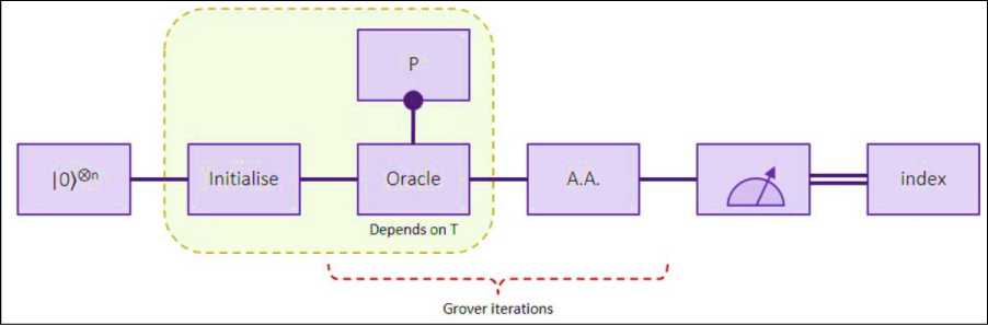
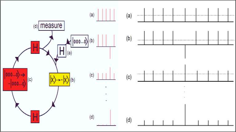
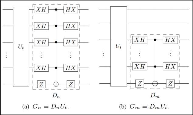
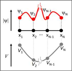
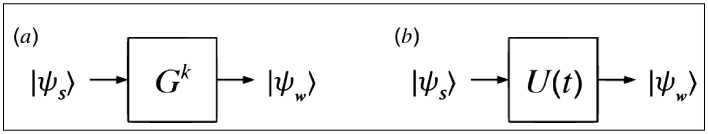
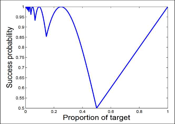
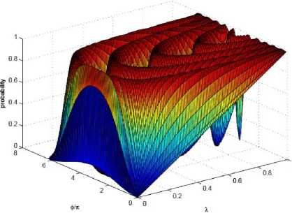
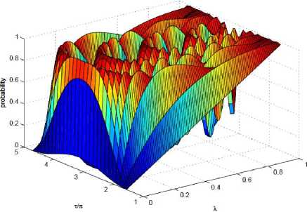
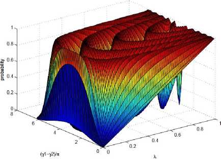
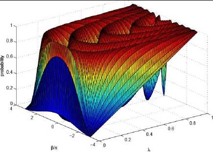
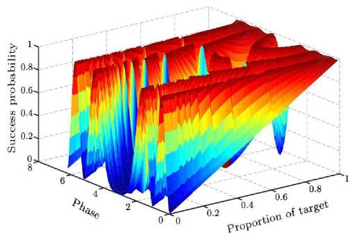
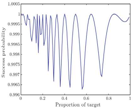
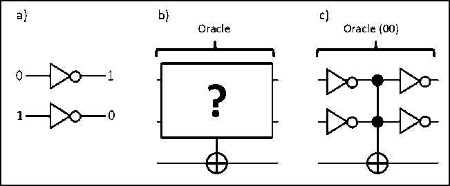
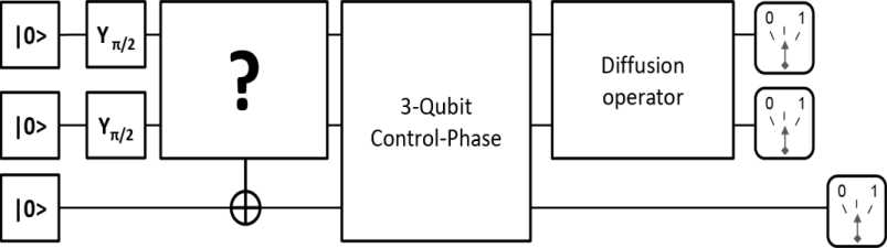
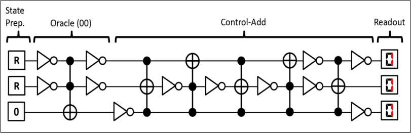
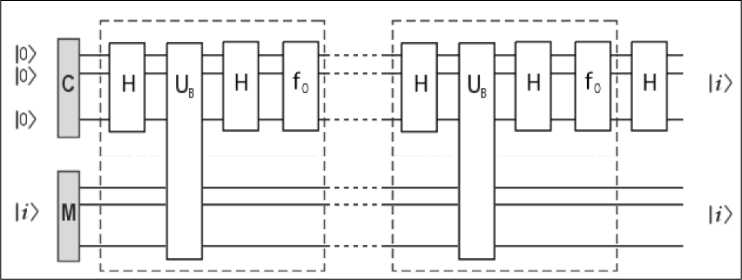
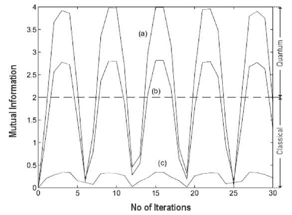
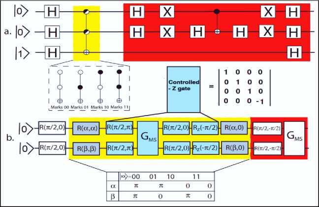

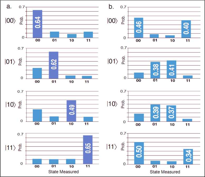
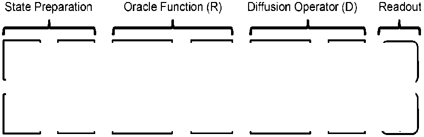
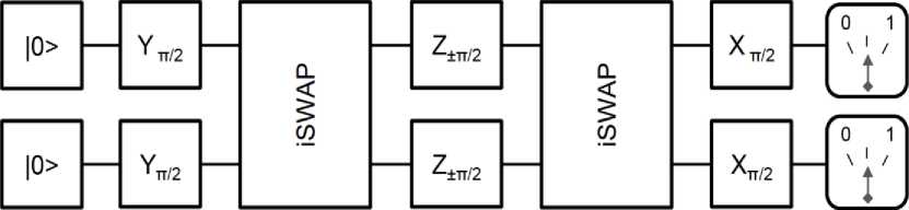
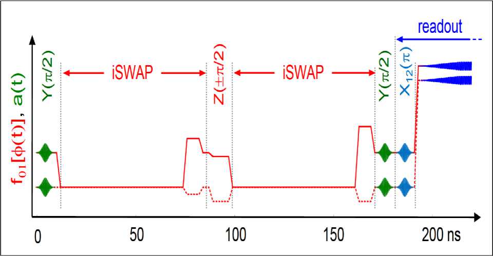
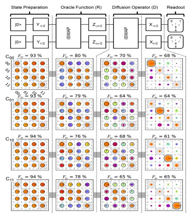

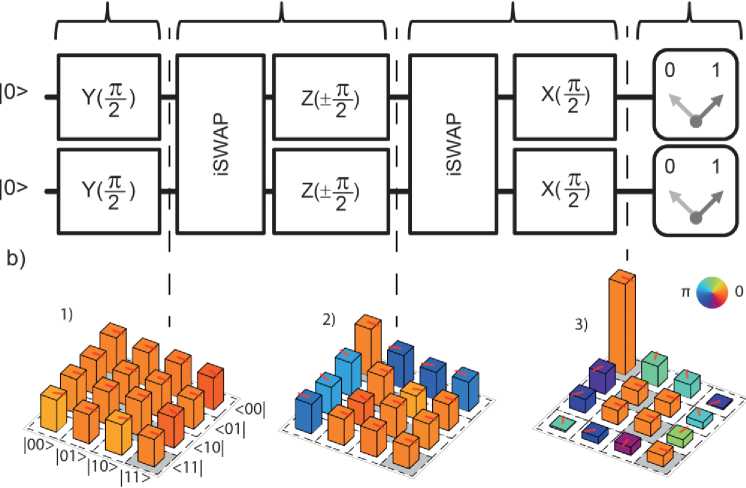
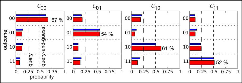
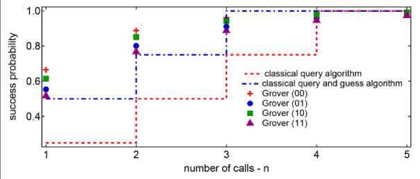
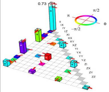
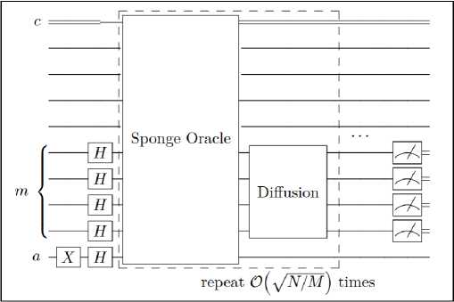
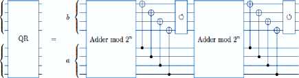
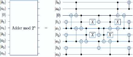
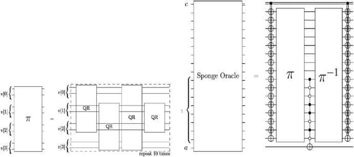
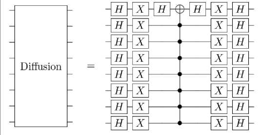
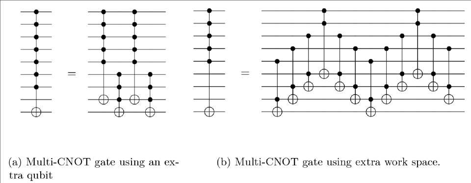
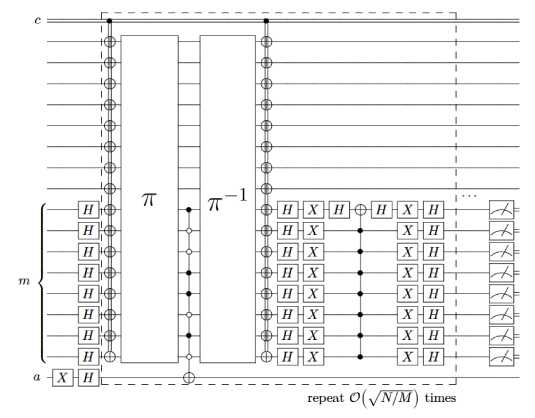

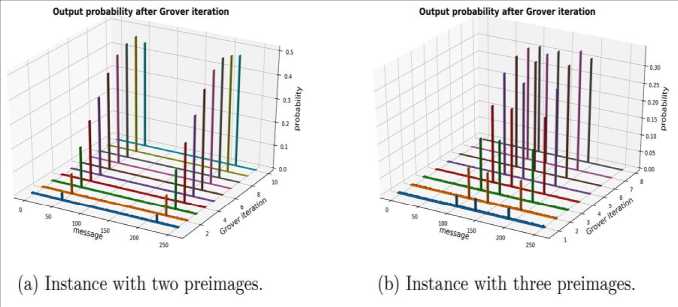
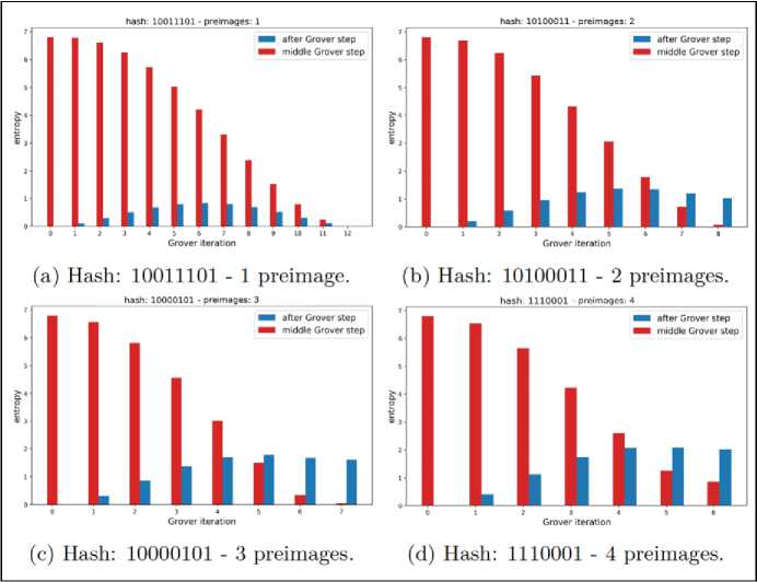
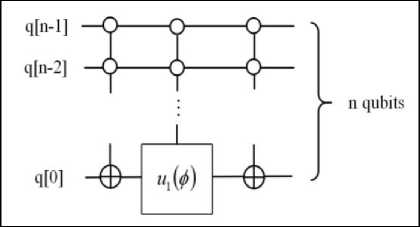
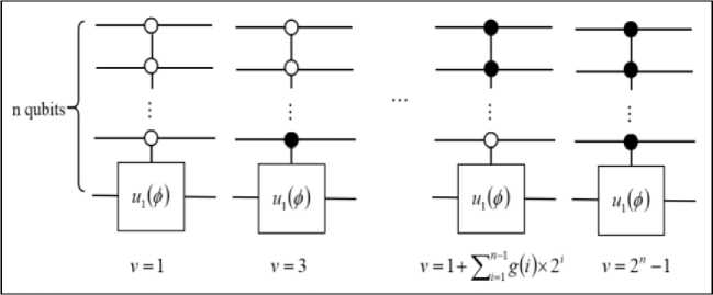
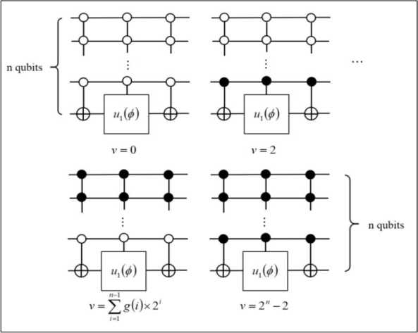
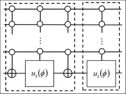
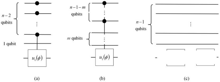
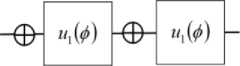
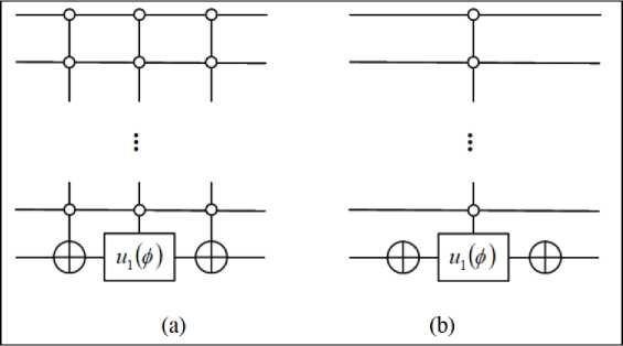
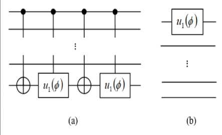
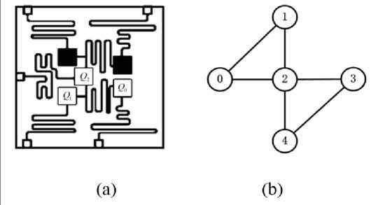
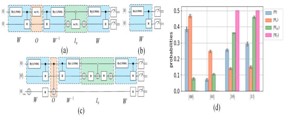
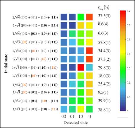
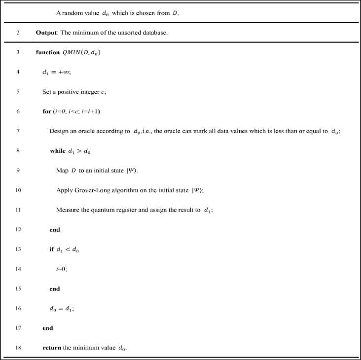
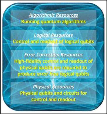
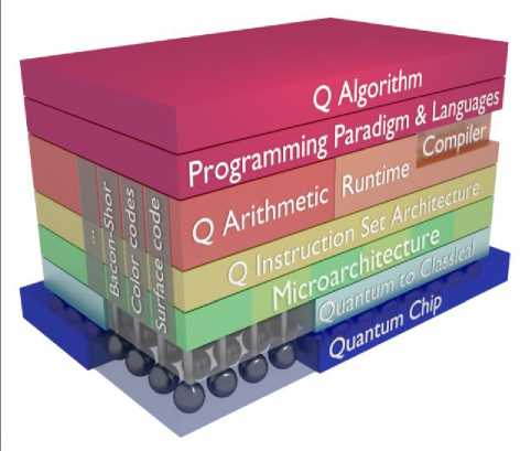
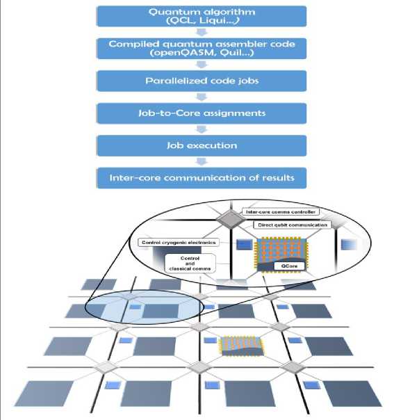
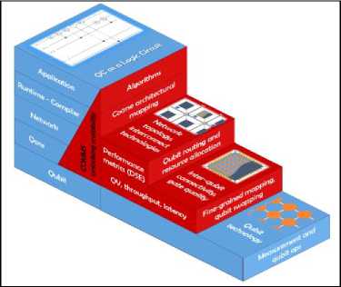
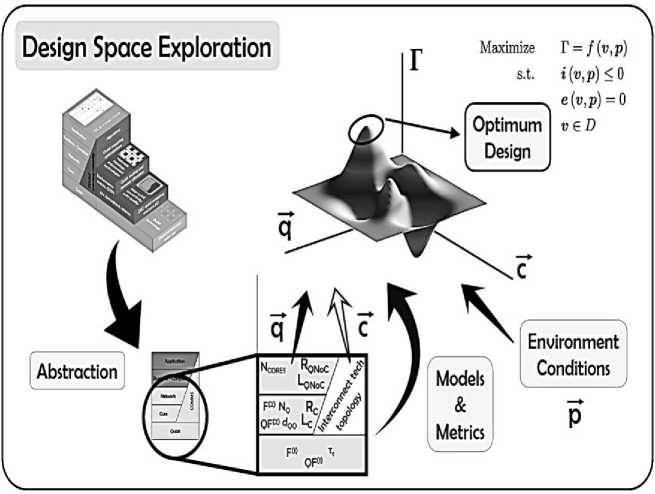
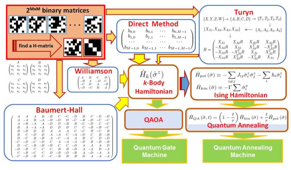
References Modelling of Grover's quantum search algorithms: implementations of simple quantum simulators on classical computers
- A Fixed-Phase Quantum Search Algorithm with More Flexible Behavior / Х Li [et al.] // J. of Quantum Information Science. – 2012. – No 2. – Pp. 28-34.
- Fixed-point quantum search with an optimal number of queries / T. Yoder [et al.] // arXiv:1409.3305v2 [quant-ph]. – 24 Nov 2014.
- Zhang, K., Korepin, V. E. Depth optimization of quantum search algorithms beyond Grover’s algorithm // arXiv:1908.04171v3 [quant-ph]. – 27 Mar 2020.
- Research on phases of Grover-type algorithms / B.-W. Ma [et al.] // arXiv:1801.07369v1 [quant-ph]. – 23 Jan 2018.
- Operating Quantum States in Single Magnetic Molecules: Implementation of Grover’s Quantum Algo-rithm / C. Godfrin [et al.] // arXiv:1710.11229v2 [quant-ph]. – 28 Nov 2017.
- A Four-Phase Improvement of Grover’s Algorithm / B.-W. Ma [et al.] // CHIN. PHYS. LETT. – 2017. – Vol. 34. – No.7. – Pp. 07030.
- Bose, S., Rallan, L., Vedral, V. Communication Capacity of Quantum Computation // Phys. Rev. Lett. – 2000. – Vol. 85. – Pp. 5448. (available: arXiv: 0003072v1 [quant-ph]. – 17 Mar 2000).
- Grover, L. From Schrödinger’s Equation to the Quantum Search Algorithm // arXiv: 0109116 [quant-ph]. – 22 Sep 2001.
- Martin-Delgado, M. A. The Schrodinger Equation, Reversibility and the Grover Algorithm // arXiv: /0412130v1 [quant-ph]. – 16 Dec 2004.
- Quantum Algorithm Design: Techniques and Applications / C. SHA [et al.] // J Syst Sci Complex. – 2019. – Vol. 32. – Pp. 375–452.
- Bausch, J. Fast Black-Box Quantum State Preparation // arXiv:2009.10709v1 [quant-ph]. – 22 Sep 2020.
- Meyer, D. A., Wong, T. G. Nonlinear quantum search using the Gross-Pitaevskii equation // New Jour-nal of Physics. – 2013. – Vol. 15. – No 6. – Pp. 063014.
- Wong, T. G. Nonlinear Quantum Search. A dissertation submitted in partial satisfaction of the require-ments for the degree Doctor of Philosophy in Physics. – University of California, San Diego. – 2014.
- Meyer, D. A., Wong, T. G. Quantum search with general nonlinearities // Physical rewiew. – 2014. – Vol. A 89. – Pp. 012312.
- Sarkar, A. Quantum Algorithms for pattern-matching in genomic sequences // Master of Science in Computer Engineering at the Delft University of Technology. – 2018.
- Quantum Simulation Logic, Oracles, and the Quantum Advantage / N. Johansson [et al.] // Entropy. – 2019. – Vol. 21. – Pp. 800 [doi:10.3390/e21080800].
- Nonlinear quantum search via coined quantum walks / B. Herzo [et al.] // arXiv:2009.07800v1 [quant-ph]. – 16 Sep 2020.
- Saleh, S. Q., Younes, A. Analyzing the reliability of quantum amplitude amplification techniques in the presence of noise // Electronic Journal of Mathematical Analysis and Applications. – 2020. – Vol. 8. – No 1. – Pp. 162–181.
- Pati, A. K. Super Quantum Search Algorithm with Weak Value Amplification and Postselection // arXiv:1910.12390v2 [quant-ph]. – 4 Nov 2019.
- Characterization of exact one-query quantum algorithms / W. Chen [et al.] // arXiv:1912.03493v2 [quant-ph]. – 23 Feb 2020.
- Characterization of exact one-query quantum algorithms (ii): for partial functions / Z. Ye [et al.] // arXiv:2008.11998v1 [quant-ph]. – 27 Aug 2020.
- A multi-step quantum algorithm for solving problems with a special structure / H. Wang [et al.] // arXiv:1912.06959v2 [quant-ph]. – 20 Aug 2020.
- Hunt, S., Gadouleau, M. Grover’s Algorithm and Many-Valued Quantum Logic // arXiv:2001.06316v1 [cs.DS]. – 17 Jan 2020.
- Quantum Search with Prior Knowledge / X. He [et al.] // arXiv:2009.08721v1 [quant-ph]. – 18 Sep 2020.
- An Optimized Quantum Maximum or Minimum Searching Algorithm and its Circuits / Y. Chen [et al.] // arXiv:1908.0794308721v1 [quant-ph]. – 18 Sep 2019.
- Tsurumaru, T. Equivalence of three quantum algorithms: Privacy amplification, error correction, and data compression // arXiv:2009.08823v1 [quant-ph]. – 18 Sep 2020.
- Transition Probabilities in Generalized Quantum Search Hamiltonian Evolutions / S. Gassner [et al.] // arXiv:2002.02242v1 [quant-ph]. – 6 Feb 2020.
- Optimizing Quantum Search Using a Generalized Version of Grover’s Algorithm / A. Gilliam [et al.] // arXiv:2005.06468v2 [quant-ph]. – 26 May 2020.
- Introducing structure to expedite quantum search / M. Brianski [et al.] // arXiv:2006.05828v1 [quant-ph]. – 10 Jun 2020.
- Quantum Search for Scaled Hash Function Preimages / S. Ramos-Calderer [et al.] // arXiv:2009.00621v1 [quant-ph]. – 1 Sep 2020.
- Number Partitioning with Grover’s Algorithm in Central Spin Systems / G. Anikeev [et al.] // arXiv:2009.05549v1 [quant-ph]. – 11 Sep 2020.
- Tutorial: Gate-based superconducting quantum computing / S. Kwon [et al.] // arXiv:2009.08021v1 [quant-ph]. – 17 Sep 2020.
- Grover Mixers for QAOA: Shifting Complexity from Mixer Design to State Preparation / A. Bärtschi [et al.] // arXiv:2006.00354v1 [quant-ph]. – 30 May 2020.
- Benchmarking 16-element quantum search algorithms on IBM quantum processors / J. Gwinner [et al.] // arXiv:2007.06539v1 [quant-ph]. – 13 Jul 2020.
- Quantum Circuits for Sparse Isometries / E. Malvetti [et al.] // arXiv:2006.00016v1 [quant-ph]. – 29 May 2020.
- Brickman, K.-A. Implementation of Grover’s quantum search algorithm with two trapped cadmium ions // A dissertation submitted in partial fulfillment of the requirements for the degree of Doctor of Philoso-phy (Physics) in The University of Michigan. – 2007.
- Dewes, A. Demonstrating quantum speed-up with a two-transmon quantum processor. Superconductivi-ty [cond-mat.supr-con]. – Université Pierre et Marie Curie. – Paris VI, 2012.
- Quantum search for scaled Hash function preimages / S. Ramos-Calderer [et al.] // arXiv:2009.00621v1 [quant-ph]. – 1 Sep 2020.
- An Optimized Quantum Maximum or Minimum Searching Algorithm and its Circuits / Y. Chen [et al.] // arXiv: 1908.07943 [quant-ph]. – 2019.
- Qibo: a framework for quantum simulation with hardware acceleration / S. Efthymiou [et al.] // arXiv:2009.01845v1 [quant-ph]. – 3 Sep 2020.
- Introduction to Coding Quantum Algorithms: A Tutorial Series Using Qiskit / D. Koch [et al.] // arXiv:1903.04359v1 [quant-ph]. – 7 Mar 2019.
- Exploring a Double Full-Stack Communications-Enabled Architecture for Multi-Core Quantum Com-puters / S. Rodrigo [et al.] // arXiv:2009.08186v1 [quant-ph]. – 17 Sep 2020.
- Practical Quantum Computing: The value of local computation / J. R. Cruise [еt al.] // arXiv:2009.08513v1 [quant-ph]. – 17 Sep 2020.
- Suksmono, A., Minato, Yu. Finding high-order Hadamard matrices by using quantum computers // arXiv:2009.10919v1 [quant-ph]. – 23 Sep 2020.
