Modified Sparseness Controlled IPNLMS Algorithm Based on l_1, l_2 and l_∞ Norms

E cho cancellation in telecommunication network requires identification of unknown echo path impulse response. The length of network echo path is typically in the range between 32 and 128 milliseconds, which is characterized by bulk delay depending on network loading, encoding and jitter delay [1]. Because of this, “active” region of echo path is in the range between 8

and 12 milliseconds, so it contains mainly “inactive” components where the coefficient magnitudes are close to zero, making the impulse response more sparse. In general, adaptive filters have been used to estimate the unknown echo path by using algorithm such as normalized least-mean-square NLMS. But, as the length of echo paths are more, NLMS requires more number of taps (up to 1024 taps) which will make the convergence of NLMS becomes poor.

Several approaches have been proposed over recent years to get better performance than NLMS for Network echo cancellation (NEC). These include Variable step size (VSS) algorithms,[2] [3] [4] partial update adaptive filtering techniques[5][6] and sub-band adaptive filtering (SAF) techniques.[7] These approaches aim to address the issues in echo cancellation including the performance with colored input signals and time varying echo paths and a computational complexity to name but a few. In contrast to these algorithms, sparse adaptive algorithms have been developed to address the performance of adaptive filters sparse system identification.

The first sparse adaptive algorithm for (NEC) is proportionate normalized least-mean-square (PNLMS)[8] in which each filter coefficient is updated independently of others, by adjusting the adaptation step size in proportion to the estimated filter coefficient. It is known that PNLMS has fast initial convergence rate.

This paper is organized as follows, in section II explains about the echo cancellation process by using recent algorithms. Section III explains about the acoustic impulse response and section IV gives about adaptive echo cancellation methods, Section V and VI gives the information about Sparse Adaptive filters and their algorithms respectively, Sections VII,VIII,IX explains about existing sparse adaptive filters, sparseness measure and   sparse impulse response generator respectively and the section X gives the various algorithms which are used to measure sparseness and their performance and in Section XI presented experimental procedure and the robust method which is the new approach with result performance is presented in section XII and this paper is summarized and concluded in section X.

• II.    ECHO CANCELLATION

Among the wide range of adaptive filtering applications, echo cancellation is likely the most interesting and challenging one. The original idea of this application appeared in the sixties [9], and it can be considered as a real milestone in telecommunication systems. A general scheme for echo cancellation is depicted in Fig.1. In both network and acoustic echo cancellation contexts [10] it is interesting to notice that the scheme from Fig.1 can be interpreted as a combination of two classes of adaptive system configurations, according to the adaptive filter theory [11]. First, it represents a “system identification” configuration because the goal is to identify an unknown system (i.e., the echo path) with its output corrupted by an apparently “undesired” signal (i.e., the near-end signal). But it also can be viewed as an “interference cancelling” configuration, aiming to recover a “useful” signal (i.e., the near-end signal) corrupted by an undesired perturbation (i.e., the echo signal); consequently, the “useful” signal should be recovered from the error signal of the adaptive filter.

Each of the previously addressed problems implies some special requirements for the adaptive algorithms used for echo cancellation. Summarizing, the “ideal” algorithms should have a high convergence rate and good tracking capabilities (in order to deal with the high length and time varying nature of the echo path impulse responses) but achieving low mis adjustment.

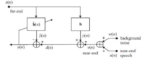
Figure 1 : General Configuration of Echo Cancellation

These issues should be obtained despite the non-stationary character of the input signal (i.e., speech). Also, these algorithms should be robust against the nearend signal variations, e.g., background noise variations and double talk. Finally, its computational complexity should be moderate, providing both efficient and low cost real-time implementation. Even if the literature of adaptive filters contains a lot of very interesting and useful algorithms [12], there is not an adaptive algorithm that satisfies all the previous requirements.

Different types of adaptive filters have been involved in the context of echo cancellation. One of the most popular is the normalized least-mean-square (NLMS)

algorithm. Also, the affine projection algorithm (APA) [originally proposed in (12)] and some of its versions, e.g., [13], [14], were found to be very attractive choices for echo cancellation. However, there is still a need to improve the performance of these algorithms for echo cancellation. More importantly, it is necessary to find some way to increase the convergence rate and tracking of the algorithms since it is known that the performance of both NLMS and APA are limited for high length adaptive filters.

• III.    ACOUSTIC IMPULSE RESPONSE (AIR)

When a sound is generated in a room, the listener will first hear the sound via the direct path from the source. Shortly after, the listener will hear the reflections of the sound off the walls which will be attenuated, as shown in Fig. 2.

Each reflection will then in turn be further delayed and attenuated as the sound is reflected again and again off the walls. Further examination of the impulse response of a room yields the observation that the sound decays at an exponential rate. Therefore, the impulse response of the room shown above may be similar to Fig. 3.

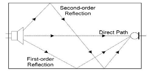
Figure 2 : A Visual Example of how sound propagates through room

The echoes effects can be reduced by having absorbers around the wall. In the case, the impulse response has less active coefficients, as depicted in Fig. 4. The latter impulse response is said to be more sparse system than the former, due to the majority of its filter taps are inactive.

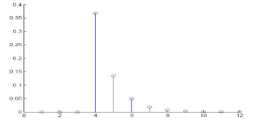
Figure 3 : Impulse response of the room shown in Fig. 2

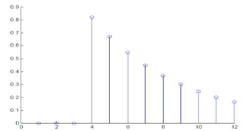
Figure 4 : Sparse impulse response of the room in the presence of echo absorbers

• IV.    THE ADAPTIVE ECHO CANCELLATION PROCESS

Fig.5. shows an acoustic echo canceller set-up by employing an adaptive filter.

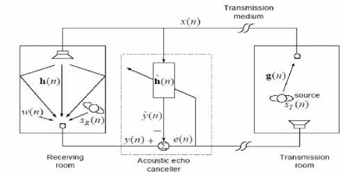
Figure 5 : Single Channel Echo Cancellation

In this paper, [ ] T denotes matrix transpose and E [ ] signifies mathematical expectation operator. Scalars are also indicated in plain lowercase, vectors in bold lowercase and matrices in bold uppercase. [27]

Notations and definitions:

• g (n) = impulse response of transmission room

= [g 0 (n) g 1 (n) g 2 (n) ……g Lt-1 (n)]^T Where L t is the length of g (n)

h (n) = impulse response of receiving room

= [h 0 (n) h 1 (n) h 2 (n) ……h Lr-1 (n)]^T Where L r is the length of h (n)

h (n)= impulse response of adaptive filter

= [h^{^} 0 (n) h^{^} 1 (n) h^{^} 2 (n) …… h^{^} L-1 (n)]^T

Where L is the length of h (n)

x (n)= input signal to the adaptive filter and the receiving room system

= [x(n) x(n-1) ... x(n-L+1)]T

S T (n) = transmission room source signal

S R (n) = Receiving room source signal

w (n) = Noise signal in Receiving room

The receiver attached in the transmission room (right hand side in fig. (2) picks up the a time varying signal x(n) from a speech source ST(n) (far-end speaker) via impulse response of the transmission room g(n). The input signal x(n) is then transmitted to the loudspeaker in the near-end receiving room. The receiving room's microphone receives the desired signal y(n) which is the convoluted sum of the input signal and the impulse response of the receiving room h(n) along with near-end speech signal and some additive noise. Therefore, yn) = hT(n)x(n) + w(n) + Sr(h) (1)

In absence of echo canceller, the received signal y(n) will be transmitted back to the origin with some delay. In the presence of an adaptive echo canceller, its objective is to estimate h(n) by taking into account the error signal e(n) at each iteration, where the e(n) is defined as e (n) = Output from the receiver room system- output from the adaptive filter

=y(n)-y^(n)                                    (2)

= [ h ^T (n)- h ¹ (n)] x (n)+w(n)+S R (n)

• •    The length of h (n), L_r is same as the length of h (n), L. In a reality, the length of the adaptive filter is less than the receiving room impulse responses. This is due to the fact that the computational complexity of an adaptive algorithm increases monotonically with the length of the adaptive filter. Therefore, L must be long enough to achieve a low system mismatch and computational complexity.

• •    There is no noise signal in the receiving room, w (n) = 0

• •    There is no source signal in the receiving room, S R (n) = 0, i.e., no doubletalk is present.

• •    A transversal finite impulse response (FIR) filter configuration is used, as shown in fig. 6, due to its stability characteristics.

• •    For effective echo cancellation, e(n) must be significantly smaller in each iteration, as the filter coefficients converges to the unknown true impulse response h(n). Several adaptive algorithms are available for the weighs update and they generally exchange increased complexity for improved performance.

Therefore Echo cancellers can be potentially employed in telecommunication systems so that the undesired echoes, both acoustic and hybrid, can be diminished.

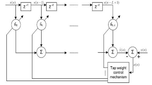
Figure 6 : Adaptive transversal FIR Filter

• V.    SPARSE ADAPTIVE FILTERS

The main goal in echo cancellation is to identify an unknown system, i.e., the echo path, providing at the output of the adaptive filter a replica of the echo. Nevertheless, the echo paths (for both network and acoustic echo cancellation scenarios) have a specific property, which can be used in order to help the adaptation process. The sparseness of an acoustic impulse response[15] is more problematic because it depends on many factors, e.g., reverberation time, the distance between loudspeaker and microphone, different changes in the environment (e.g., temperature or pressure), however, the acoustic echo paths are in general less sparse as compared to their network counterparts, but their sparseness can also be exploited.

Even if the idea of exploiting the sparseness character of the systems has appeared in the nineties, e.g.,[16],[17], [18], the proportionate NLMS (PNLMS) algorithm[19] proposed by Duttweiler a decade ago, was one of the first“true”proportionate-type algorithms and maybe the most referred one. As compared to its predecessors, the update rule of the PNLMS algorithm is based only on the current adaptive filter estimate, requiring no a priori information about the echo path. However, the PNLMS algorithm was developed in an “intuitively” manner, because the equations used to calculate the step-size control factors are not based on any optimization criteria but are designed in an ad-hoc way. For this reason, after an initial fast convergence phase, the convergence rate of the PNLMS algorithm significantly slows down. Besides, it is sensitive to the sparseness degree of the system, i.e., the convergence rate is reduced when the echo paths are not very sparse. In order to deal with these problems, many proportionate-type algorithms were developed in the last decade. The overall goal of this paper is to present and analyse the most important sparse adaptive filters, in order to outline their capabilities and performances in the context of echo cancellation. In view of this paper reviews the basic proportionate-type NLMS adaptive filters, the classical PNLMS [19], the improved PNLMS [20], and other related algorithms are discussed. The exponentiated gradient (EG) algorithms [21] and their connections with the basic sparse adaptive filters are presented. Some of the most recent developments in the field, including the mu-law [22],  [23] and other new PNLMS-type algorithms are also included. A variable step-size PNLMS-type algorithm is also analysed for aiming to better compromise between the conflicting requirements of fast convergence and low maladjustments encountered in the classical versions. Which further improve the performance of the PNLMS-type algorithms [26].

An impulse response can be considered “sparse” if a large fraction of its energy is concentrated in a small fraction of its duration. Adaptive system identification is a particularly challenging problem for sparse systems. [36] An application of sparse system identification which is of current interest is packet-switched network echo cancellation. The increasing popularity of packet-switched telephony has led to a need for the integration of older analog systems with, for example, IP or ATM networks. Network gateways enable the interconnection of such networks and provide echo cancellation. In such systems, the hybrid echo response is delayed by an unknown bulk delay due to propagation through the network. The overall effect is therefore that an “active” region associated with the true hybrid echo response occurs with an unknown delay within an overall response window that has to be sufficiently long to accommodate the worst case bulk delay.

In the context of Networking and acoustic echo cancellation the convergence performance, computational complexity of the existing sparse adaptive filters and the performance of sparseness measure of improvement is analysed .Finally the recent algorithms of sparse adaptive filters which were mentioned in section X are discussed. It has been observed that the proposed algorithms Sparseness controlled µ-Law Proportionate NLMS (SC-MPNLMS) and Sparseness controlled- Improved Proportionate NLMS (SC-IPNLMS)[24] and the (MSC-IPNLMS) are robust to variations in the level of sparseness in AIR with only a modest increase in computational complexity[27].

• VI.    SPARSE ADAPTIVE FILTER ALGORITHMS

A sparse impulse response has most of its components with small or zero magnitude and can be found in telephone networks. Due to the presence of bulk delays in the path only 8-10% exhibits an active region. Fig.7 shows a typical sparse impulse response, which can be realized in reality.

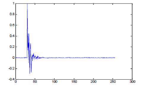
Figure 7 : An example of a sparse impulse response exists in telephone networks.

The NLMS algorithm does not take into account this feature when it presents in a system and therefore performs inadequately. This is because [24].

• •    The need to adapt a relatively long filter

• •    The unavoidable adaptation noise occur at the inactive region of the tap weights

  

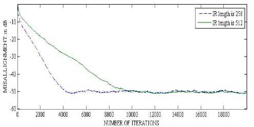
  Figure 8 : Convergence of NLMS when Filter Length changes from 256 to 512.

  
  

coefficients in an efficient way that the step size is proportional to the size of the filter coefficients. This is resulted to adjust the active coefficients faster than the non-active ones. Therefore, the overall convergence time is reduced.

VIII. SPARSNESS MEASURE

Degree of sparseness can be qualitatively referred as a range of strongly dispersive to strongly sparse. Quantitatively, the sparseness of an impulse response can be measured by the following sparseness measure

While in the NLMS, the adaptation step is same for all components of the filter, in the sparse algorithms, such as PNLMS, IPNLMS and MPNLMS, adaptive step sizes are calculated from the last estimate of the filter coefficients in an efficient way that the step size is proportional to the size of the filter coefficients. This is resulted to adjust the active coefficients faster than the non-active ones. Therefore, the overall convergence time is reduced.

£( h ) =

L

L - VL

h ( n ) ₁

L h ( n ) ₂

Where from equation number 3

L = 1     2

IIh(n1 =VEl=0 hl (n)

VII. EXISTING SPARSE ADAPTIVE FILTER ALGORITHMS

The method of steepest descent avoids the direct matrix inversion inherent in the Wiener [15].This paper gives the in detailed information by studying the most common approach to sparse adaptive filtering, the stochastic gradient based algorithms. And several modifications to this algorithm, are made in order to cope with practical constraints, and are discussed in. Since a wide variety of algorithms are available in the survey, this paper defines and analyses the existing sparse adaptive filter and their performances using simulation results [25] of their different subjective measures and computational requirements. Stochastic gradient based algorithms do not provide an exact solution to the problem of minimizing the MSE as the steepest descent approach, rather approximates the solution. However, the requirement for stationary input or knowledge of autocorrelation matrix, and the crosscorrelation vector, in steepest descent approach are circumvented in the algorithms [15].

This type of algorithms are widely used in various applications of adaptive filtering due to its low computational simplicity, proof of convergence in the stationary environment, unbiased convergence in the mean to the Wiener solution and stable behavior in the finite-precision arithmetic implementations .

While in the NLMS, the adaptation step is same for all components of the filter, in the sparse algorithms, such as PNLMS, IPNLMS and MPNLMS, adaptive step sizes are calculated from the last estimate of the filter

IX. SPARSE IMPULSE RESPONSE GENERATOR

Sparseness of impulse responses for Network and acoustic echo cancellation can be studied by generating synthetic impulses using random sequences. This can be achieved by first defining an L×1 vector

U x i =k_{X 1}    1   e ^{- 1}/ ^Ф    e - 2 ^Ф...... e⁴L u ^{- 1)}/ ^Ф ]" (4)

L - 1

II ^{h ( n} )ll₂ = E h ^{( n} ) l = 0

Where the leading zeros with length Lp models the length of the bulk delay and Lu = L – Lp is the length of the decaying window which can be controlled by ψ. Smaller the ψ value yields more sparse system.

Defining a Lu × 1 vector b as a zero mean white Gaussian noise (WGN) sequence with variance σ b ², the L × 1 synthetic impulse response can then be expressed as

BLu x Lu = diag {b},

	\oLxL   oLXa
h ( n ) =	p pp      ^ x Рц _ 0 L u x L p     B L u x L pu _	u + P

Where the L × 1 vector p ensures elements in the ‘inactive’ region are small but non-zero and is an independent zero means WGN sequence with variance _σp 2

Fig 2.shows two impulse responses that can be attained using this approach, by setting the impulse length L =512, the bulk delay length L p =32 and ψ to 8(more sparse), 20, 50 and 100(more sparse).

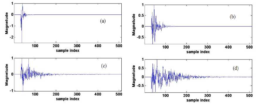
Figure 9 : Impulse responses controlled using (a) ψ = 8, (b) ψ = 20, (c) ψ =50 and (d) ψ =80 giving sparseness measure (a) ξ = 0.905,(b) ξ = 0.809, (c) ξ = 0.667 and (d) ξ = 0.

• X. SPARSENESS MEASURE ALGORITHMS

When Impulse response is less sparse or dense then NLMS works better than PNLMS.

• A. Proportionate Normalised Least Mean Square (Pnlms)

One of the first sparse adaptive filtering algorithms considered as a milestone for NEC is PNLMS, in which each filter coefficient is updated with an independent step-size that is linearly proportional to the magnitude of that estimated filter coefficient. It is well known that PNLMS has very fast initial convergence for sparse impulse responses after which its convergence rate reduces significantly, sometimes resulting in a slower overall convergence than NLMS.

In order to track sparse impulse response faster Proportionate NLMS (PNLMS) was introduced from the NLMS equation. The coefficient update equation of the PNLMS is slightly differ from NLMS with the extra step size update matrix Q as shown below and the rest of the terms are carried over from NLMS.

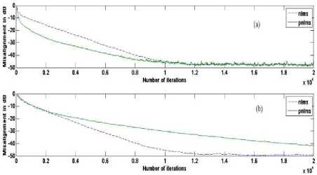
Fig.10: Relative convergence of NLMS, PNLMS using WGN input for (a) ψ=8 and (b) ψ=80 Initial step size µ=0.3 for both NLMS and PNLMS

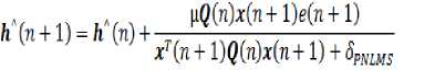
Where 6PNLMS = cst.a^/L

Q(tl) = diay{q_o(n),........<7z_-iOO}

B.Improved Proportionate Normalised Least Mean

Sqaure (Ipnlms )

Controls the step size. These control matrix elements can be expressed as

Parameters ρ and γ have typical values of 5 / L and 0.01 [8], respectively. The former prevents coefficients from stalling when they are much smaller than the largest coefficient and the latter prevents        from stalling during initialization stage.

This Algorithm shows fast initial convergence phase and then convergence rate of the PNLMS algorithm significantly slows down. Besides, it is sensitive to the sparseness degree of the system, i.e., the convergence rate is reduced when the echo paths are not very sparse.

An improvement of PNLMS is the IPNLMS algorithm, which employs a combination of proportionate (PNLMS) and non-proportionate (NLMS) updating technique, with the relative significance of each controlled by a factor α. gl(n) of PNLMS is updated as follows for the IPNLMS approach.

Where ∈ is a small positive number. Good choice for α are 0, -0.5 and -0.75. The regularization parameter should be taken as follows, in order to achieve the same steady state misalignment compare to that of NLMS using same step size.

In the above, first Equation is made up of the sum of two terms, where the first is a constant and the second term is a function of the weight coefficients. It can be noticed that, when α = -1 the second term becomes zero and therefore the k becomes 1/L. It means that the same update will be made to all filter coefficients regardless of their individual magnitudes. So, for this α value IPNLMS performs as NLMS. For α close to unity, the second term dominates the equation and as a result it behaves as PNLMS.

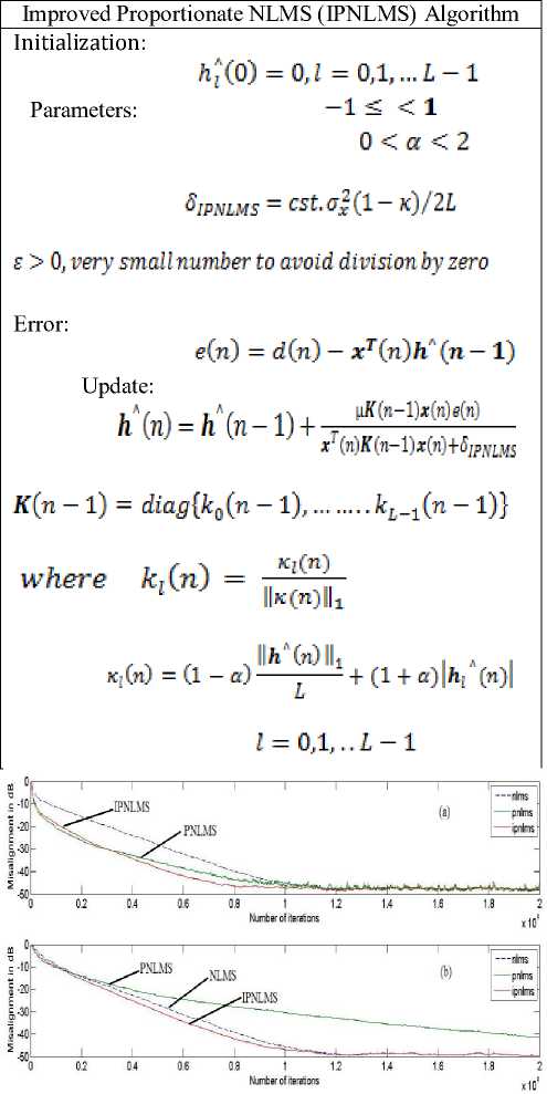
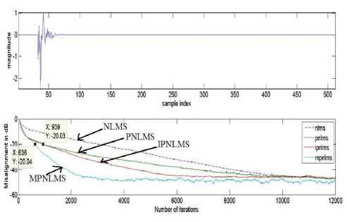
Fig.11: Relative convergence of NLMS, PNLMS and IPNLMS using WGN input for (a) ψ=8 and (b) ψ=80 Initial step size µ=0.3 for NLMS, PNLMS and IPNLMS and α=-0.75.

C.µ-Law Proportionate Nlms (Mpnlms)

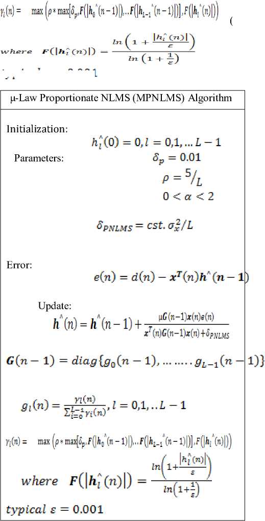
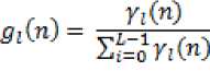
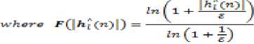
Another variant of PNLMS algorithm is µ-Law Proportionate NLMS (MPNLMS) algorithm. The MPNLMS algorithm calculates the optimal proportionate step size in order to achieve the fastest convergence during the whole adaptation process until the adaptive filter reaches its steady state. The definition for Yi GO of MPNLMS is differed as follows from that of previous proportionate algorithms.

typical £ = 0.001

The constant 1 inside the logarithm is to avoid obtaining negative infinity at the initial stage when H^ (O> = О . The denominator '- (■ + f) normalizes *<|АГООП to be in the range [0, 1]. The vicinity ε is a very small positive number, and its value should be chosen based on the noise level. ε = 0.001 is a good choice for echo cancellation, as the echo below -60 dB is negligible.

It can be noted that a linear function рОО = 1 - ^(тГ) also achieves our desired function.

The choice of λ is important. As can be seen from above fig. that, larger value of λ will cause the proposed SC-MPNLMS to inherit more of the MPNLMS properties compared to NLMS giving good convergence performance when Impulse response (IR) is sparse. On the other hand, when IR is dispersive, λ must be small for good convergence performance. Hence, as shown in above fig., that a good compromise is given by λ=6.

In addition, we note that when n=0, Н^'СО)||2 = о and hence, to prevent division by zero or small number,

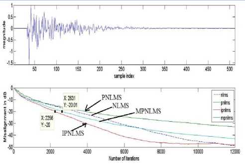
Fig.12: Relative convergence of NLMS, PNLMS, IPNLMS and MPNLMS using WGN input for (a) ψ=8 and (b) ψ=80 Initial step size µ=0.3 for NLMS, PNLMS, IPNLMS and MPNLMS and α=-0.75.

V (™) can be computed for      . When

, we

АС”) = -•/ set

• E.    Sparseness Controlled µ-Law Proportionate Nlms (Sc-Mpnlms) Algorithm

Initialization: ^(0)=0,1 = ПД„1-1 Parameters:

8р = 0.01     0 < а < 2

6$c-mpnlms — cst.o^/L

Error: e(n) = d(n) - *r(n)h' (n-1)

Update: h' (n) - hA(n - 1) + r ^"-^^--- x' (n)G(n-l)x(n)+6sC-MPNLMS

D.Sparseness Controlled Mpnlms (Sc-Mpnlms) Algorithm

In order to address the problem of slow convergence in PNLMS and MPNLMS for dispersive AIR, we require the 0г Ста) to be robust to the sparseness of the impulse response. Several choices can be employed to obtain the desired effect of achieving a high convergence when С ■ о-э is small when estimating dispersive AIRs. We consider an example function

The variation of <-С") in MPNLMS for the exponential function is as shown in fig. below for the cases is 4, 6 and 8.

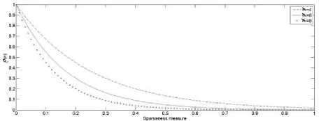
Figure 13: Variation of ρ against sparseness measure^Гоо of impulse response for different values of λ

• F.    Sparseness Controlled Ipnlm (Sc-Ipnlms) Algorithm

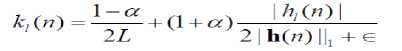
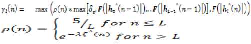
A different approach, compared to SC-MPNLMS, is chosen to incorporate sparseness-control into the IPNLMS algorithm (SC-IPNLMS) because, two terms are employed in IPNLMS for control of the mixture between proportionate and NLMS updates. The proposed SC-IPNLMS improves the performance of the IPNLMS by expressing ql(n) for n ≥ L as

I Г1-0.5е(п)1 (l-osa-ip) . Г1+ 0.5e(n)l (l+osc-ip)IMn)| gr(n|= ----------- ------------ + ----------- ----—-------------.

^           2£               L         2||h(n)||i + 5]p

As can be seen, for large ξ^(n) when the impulse response is sparse, the algorithm allocates more weight to the proportionate term of IPNLMS. For comparatively less sparse impulse responses, the algorithm aims to achieve the convergence of NLMS by applying a higher weighting to the NLMS term. An empirically chosen weighting of 0.5 in the above equation is included to balance the performance between sparse and dispersive cases, which could be further optimized for a specific application. In addition, normalization by L is introduced to reduce significant coefficient noise when the effective step-size is large for sparse AIRs with high ξ^(n).

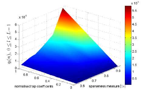
Figure 14: Magnitude of ql(n) for 0 ≤ l ≤ L-1 against the magnitude of coefficients АГ (m) in SC-IPNLMS and different sparseness measures of 8 systems.

Fig.12. illustrates the step-size control elements ql(n) for SC-IPNLMS in estimating different unknown AIRs. As can be seen, for dispersive AIRs, SC-IPNLMS allocates a uniform step-size across Й-Г OO while, for sparse AIRs, the algorithm distributes ql(n) proportionally to the magnitude of the coefficients. As a result of this distribution, the SC- IPNLMS algorithm varies the degree of NLMS and proportionate adaptations according to the nature of the AIRs.

Sparseness controlled Improved Proportionate NLMS (SC-IPNLMS) Algorithm.

Initialization: ^(0) = 0,Z = 0,l,...i-l

Parameters: ^asc-ip - “0.75

• XI.    EXPERIMENTALS RESULTS

Experimental Setup:

Throughout the simulations, algorithms were tested using a zero mean WGN and a male speech signal as inputs while another WGN sequence w(n) was added to give an SNR of 20 dB. The length of the adaptive filter L = 1024 was assumed to be equivalent to that of the unknown system. The sparseness measure of these AIRs giving ξ(n) = 0.83 and ξ(n) = 0.59 respectively.

Convergence Performance of SC-MPNLMS for AEC

Fig. 13 and 14 illustrates the performance of NLMS, MPNLMS and SC-MPNLMS using WGN as the input signal. Step sizes are adjusted to achieve the same steady state misalignment for all algorithms. This corresponds to    µNLMS=0.3,    µMPNLMS=0.25,    µSC-

MPNLMS=0.35. The value of λ=6 was used for SC-MPNLMS. As can be seen from the result, the SC-MPNLMS algorithm attains approximately 9 dB improvement in normalized misalignment during initial convergence compared to NLMS and same initial performance followed by approximately 2.5 dB improvement over MPNLMS for the sparse AIR and SC-MPNLMS achieves approximately 2.7 dB improvement compared to MPNLMS and about 5 dB better performance than NLMS for dispersive AIR.

During Sparse Impulse response.

^sc-ipnlms - ^t.a^L

Error: s(n) = i!(n)-/№‘(n-l)

Update: ft‘(n)=h"(n-l)+

l4(n-l)i(«)e(n)

3tT(«)C(«-l)lMl^-™№

Q(n- l) = dityf{q0(n-l),.....

(1 - $5нр)    (1 + «sc-ip) I ^ ИI

41 nJ = —----+ .......  . „-----

qL-i(n -!))

’SC-1PNLMS

/cm <  L

During Dispersive Impulse response :

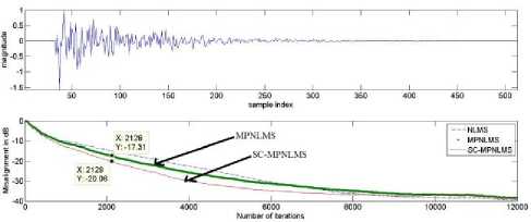
Figure 15: Relative Convergence of NLMS, MPNLMS and SC-MPNLMS when impulse response is Dispersive.

?iW=

l-d^tnjltl-^,). fl+0.5/(n)] (l+^^Ml

L

2L

2|№'М111+^ИРШ1

forn>L

The sparseness-controlled algorithms (SC-PNLMS, SC-MPNLMS and SCIPNLMS) give the overall best performance compare to their conventional methods across the range of sparseness measure. This is because

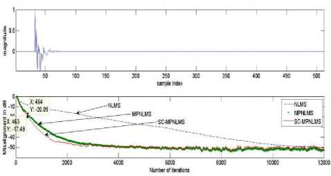
Figure 16: Relative Convergence of NLMS, MPNLMS and SC-MPNLMS when impulse response is Sparse the proposed algorithms take into account the sparseness measure of the estimated impulse response at each iteration.

• XII.    MODIFIED SPARSENESS CONTROLLED IPNLMS (MSC-IPNLMS):

In the earlier algorithms like SC-IPNLMS and SC-MPNLMS, the sparseness measure used to measure the time varying sparseness of the impulse response to be identified is based on the l1 and l2 norms. But this sparseness measure is the good representation of sparse impulse response only. So, we can improve the performance of SC-IPNLMS by incorporating another sparseness measure which is good representation of both sparse and dense impulse response. The new sparseness measure is the average of ζ 12 ( i.e. sparseness measure based on l 1 and l 2 norms) and ζ 2∞ ( i.e. sparseness measure based on l 2 and l ∞ norms). ζ 12 is a good representation of sparse impulse response where as ζ 2∞ is a good representation of dense impulse response. Hence ζ 12∞ is good representation of both sparse impulse response and dense impulse response.

Convergence Performance of MSC-IPNLMS for AEC.

Fig. 15 and 16 illustrates the performance of IPNLMS, SC-IPNLMS and MSC-IPNLMS using WGN as the input signal. Step sizes are adjusted to achieve the same steady state misalignment for all algorithms. This corresponds to IPNLMS =0.3, SC-IPNLMS =0.7, MSC-IPNLMS =0.9.

So by including ζ 12∞ in the above SC-IPNLMS algorithm in the place of ζ^, this new MSC-IPNLMS algorithm showing the improvement of 4 dB over SC-IPNLMS when impulse response is more sparse and it is showing the improvement of 8 dB when impulse response is less sparse or dense.

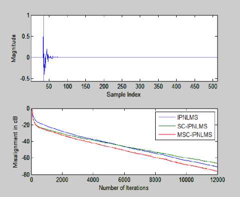
Figure 17: Relative Convergence of IPNLMS, SC-IPNLMS and MSC-IPNLMS when impulse response is Sparse.

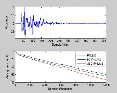
Figure 18: Relative Convergence of IPNLMS, SC-IPNLMS and MSC-IPNLMS when impulse response is Dispersive.

• XIII.    C onclusions and prospects

This paper has addressed the significant problem caused by undesirable echoes that result from coupling between the loud speakers and microphones in the near end room. The research for this work focuses on the development of the adaptive filtering algorithms for sparse and non-sparse systems, emphasizing on the achievement of fast convergence rate with relatively low computational cost.

The trade-off between convergence speed and the steady state misalignment is an important issue in this context, and can be balanced by choosing a sensible step size for the adaptive processes.

A series of experiments carried out both within and across NLMS, as well as a few other proportionate techniques, namely PNLMS, IPNLMS and MPNLMS, help to investigate their strengths and weaknesses. NLMS gives better performance in non-sparse system, whereas MPNLMS performs well in sparse impulse response. The combination of non-sparse and sparse technique, IPNLMS, exhibits an overall of better performance in all sparse levels. This identified an important factor, the sparseness measure (ξ), which affects their convergence speed.

By introducing ξ in both MPNLMS and IPNLMS, adaptive algorithms for acoustic echo cancellation can achieve fast convergence and robustness to sparse impulse response. The algorithms, known as SC-MPNLMS and SCIPNLMS, take into account this factor differently via the coefficient update function. Simulation results show that the SC-IPNLMS exhibits more robustness to sparse systems than the other techniques. And the sparseness measure ζ12 used by the SC-IPNLMS and SC-MPNLMS is a good representation of sparse impulse response, so we have replaced this with ζ12∞ which is a good representation of both sparse and dense impulse response. And the algorithm with this sparseness measure showing better performance over SC-IPNLMS in the both sparse and dense impulse response, though its computational complexity is slightly higher than the existing main stochastic algorithms, this modified algorithm perform better in all ξ levels.