Modifying one of the Machine Learning Algorithms kNN to Make it Independent of the Parameter k by Re-defining Neighbor

Author: Pushpam Kumar Sinha
Journal: International Journal of Mathematical Sciences and Computing @ijmsc
Article in issue: 4 vol.6, 2020.
Free access
When we are given a data set where in based upon the values and or characteristics of attributes each data point is assigned a class, it is known as classification. In machine learning a very simple and powerful tool to do this is the k-Nearest Neighbor (kNN) algorithm. It is based on the concept that the data points of a particular class are neighbors of each other. For a given test data or an unknown data, to find the class to which it is the neighbor one measures in kNN the Euclidean distances of the test data or the unknown data from all the data points of all the classes in the training data. Then out of the k nearest distances, where k is any number greater than or equal to 1, the class to which the test data or unknown data is the nearest most number of times is the class assigned to the test data or unknown data. In this paper, I propose a variation of kNN, which I call the ANN method (Alternative Nearest Neighbor) to distinguish it from kNN. The striking feature of ANN that makes it different from kNN is its definition of neighbor. In ANN the class from whose data points the maximum Euclidean distance of the unknown data is less than or equal to the maximum Euclidean distance between all the training data points of the class, is the class to which the unknown data is neighbor. It follows, henceforth, naturally that ANN gives a unique solution to each unknown data. Where as , in kNN the solution may vary depending on the value of the number of nearest neighbors k. So, in kNN, as k is varied the performance may vary too. But this is not the case in ANN, its performance for a particular training data is unique. For the training data [1] considered in this paper, the ANN gives 100% accurate result.
Euclidean distance, k-Nearest Neighbor, Training data, Linearly separable data, Non-linearly separable data
Short address: https://sciup.org/15017553
IDR: 15017553 | DOI: 10.5815/ijmsc.2020.04.02
Text of the scientific article Modifying one of the Machine Learning Algorithms kNN to Make it Independent of the Parameter k by Re-defining Neighbor
One of the common problems in machine learning is that of classification of objects, and one of the easiest and yet powerful tool to do this is the conventional kNN (k-Nearest Neighbor) method. The basic concept of kNN is that the objects which are similar to each other and hence belonging to one particular class tend to remain closer to each other and far from the objects of the other class. In other words the objects of the same class are neighbors of each other. Therefore, in kNN, to find out whether the two chosen data points are neighbors of each other or not, we must somehow know to measure the distance between the two data points. And the distance most commonly measured in kNN is Euclidean distance [1].
Suppose that a certain considered data set has n data points, classified into m classes, based upon p attributes. Let the i-th attribute be denoted by X [ . Then the Euclidean distance (Ed) between two data points 1 and 2 is
Ed 1-2
l^(X“ "
X i2 )2
where Хц is the value of attribute i for data point 1, and X [ 2 is the value of attribute i for data point 2
Let unknown data point be u for which we need to determine the class. We find the Ed of u from each of the n data points, and denote it Edu- j , j = 1,2, ..., n. Fix value of к, the minimum value is 1 and the maximum may be the square root of the number of known data points [1]. Once value of к is fixed, find к known data points closest to the unknown data u; the class of each of these closest data points will be the class of the unknown data point respectively. We will find the class of u finaly by majority voting of the several classes assigned to u. The performance of conventional kNN is naturally affected by the choice of к. I, in this paper, am in search of a method which is free from the parameter к and thereby its performance is not dependent on the choice of к.
Over the years there have been several advancements to the conventional kNN, and broadly the different kNN techniques are classified into Structure based kNN and Non-structure based kNN [2]. The need for providing structure to the input data points arose because of the memory limitation of the conventional kNN for very large and highly dimensional data sets. Ball-tree based algorithms (BTAs) are one of the popular structure based kNNs. In BTA nodes/balls are made enclosing all/some of the input data points of the data set. The node enclosing all the input data points of the data set is the root node, where as they including a certain subset of the data set are either the children to root node or the grandchildren to child node. In each of the node/ball, node radius is found out as the maximum distance of the pivot point from the rest of the data points enclosed inside the node. Pivot point may be any one of the data points that the node owns or it may be the centroid of the data points that the node owns. The BTAs being mention here are KNS1, KNS2 and KNS3. KNS1 is due to Uhlmann [3], while KNS2 and KNS3 are due to Liu et al [4]. KNS1 explicitly finds out the к nearest neighbors of unknown data point u (whose class is unknown), while KNS2 and KNS3 does not. Both KNS2 and KNS3 are algorithms for binary classification. KNS2 finds out how many of the к nearest neighbors of и are positive, while KNS3 finds out if at least t of the к nearest neighbors of и are positive. Thus all the three BTAs have their performance dependent upon the choice of pivot points for the nodes/balls and the value of к, and for KNS3 also on t. The method that I have developed in this paper is free from all these parameters. Though in my method too I find out the maximum distance for the input data points belonging to a particular class, but this maximum distance is not found out from the pivot point to the rest of the points in the class. There is no pivot point in my method, instead for each class I find out the maximum distance between all the data points that belongs to the class (see Section 2). I call my method the ANN (Alternative Nearest Neighbor) to distinguish it from kNN.
The other popular structure based kNNs include k-d tree [5], nearest feature line (NFL) [6], tunable metric [7], principal orthogonal search tree [8], axis search tree [9], etc.. I do not discuss these here as my method is completely different from these, and hence these are not the pre-requisites to understand my method. Moreover, these are not the stepping stones towards developing my method.
The best example of non-structure based kNN is the conventional kNN [10] which I have introduced above. Using the concept of weights, the conventional kNN underwent some change [11]. In [11] the input data points are assigned weights based on their distances from the unknown data point. However, the solution to the problem of moving unknown points in the space of known data set is different; the notable solutions are by [12], [13] (Continuous RNN), [14], etc. All these are also the non-structure based kNNs. None of these too, with the exception of conventional or classical kNN, are stepping stones towards developing my method.
-
2. The ANN method
There is no challenge to the concept of conventional kNN that similar objects are neighbors of each other or neighbors are those who are similar to each other and hence belonging to the same class. The measure of similarity mostly adopted is Euclidean distance. A natural question that the above concept raises is how close (less than or equal to a particular threshold value) should the two particular neighbors be so that if the distance between these two data points is greater than the one defining proximity between neighbors, then the two data points are not neighbors. And while developing a machine learning algorithm the answer to the above question must not be subjective. The clue to answer the above question objectively lies in the input data set of the particular classification problem itself, also, called the training data in machine learning paradigm.
The ANN method believes that there is no lower limit to how close the two neighbors can get, but there always is an upper limit to how far the two neighbors are. For a data set for which the above boundary of neighborhood has not been declared explicitly, we find the maximum distance between the data points belonging to a particular class as the farthest that the two particular data points belonging to the class can get, and this defines the boundary of neighborhood for that class. This means that for a class with I data points a combination of any two data points out of I has to be chosen and the distance between the two calculated, thereby calculating in total l (l^ 1 distances. Out of these l (l^ 1 distances the maximum defines the boundary (upper limit) of neighborhood of that class. The striking feature of ANN that makes it different from kNN is this very definition of neighbor. To be precise, in ANN the class from whose data points the maximum Euclidean distance of the unknown data is less than or equal to the maximum Euclidean distance between all the training data points of the class, is the class to which the unknown data is neighbor.
Consider a certain training data with p data points segregated into classes 1, 2 and 3 with I , m and n data points respectively based on the value of two attributes x and y.
I + m + n = p (1)
Let the boundary of neighborhood in class 1, 2 and 3 respectively (i.e. the maximum distance amongst the set of data points belonging to a particular class) be distmax [1], distmax [2] and distmax [3] respectively, the distance Ed1-2 between any two data points 1 and 2 of the training data being given by
Ed1-2 = 7 (X 1 - X 2 )2 + (У 1 - У 2 ) 2 (2)
where the symbols have usual meaning (see Section 1)
Let the unknown data or test data be u. Find the maximum distance of u from the data points in each of the class 1, 2 and 3 separately, and denote it by distmax2[1], distmax2[2] and distmax2[3] respectively. An algorithm to find distmax2[1] is for (k=1;k<=l;k++)
dist2[k]=0.0;
for (k=1;k<=l;k++)
dist2[k]=dist2[k]+sqrt((xu-xk)* (xu-xk)+ (yu-y k )* (yu-yk));
distmax2[1]=0.0;
for(k=1;k<=l;k++)
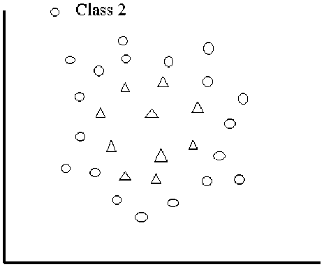
if(distmax2[1] distmax2[1]=dist2[k]; Some of the syntax used in above algorithm is that of the C/C++ programming language. 2.1 Assigning class in ANN method for the above mentioned training data 3. Example Training Data If for a certain class i only distmax2 [i] < distmax [i], we say that the unknown data or the test data belong to class i. If, however, for two classes or more than two classes, say for example class 1 and 2 here distmax2[1] < distmax[1], distmax2[2] < distmax[2] and distmax2[1] not equal to distmax2[2], the unknown data or the test data belongs to the class к (=1,2) for which distmax2[к] is minimum. If, however, for two classes or more than two classes, say for example class 1 and 2 here distmax2[1] < distmax[1], distmax2[2] < distmax[2] and distmax2[1] equal to distmax2[2], the unknown data or the test data belongs to the class к (=1,2) for which the percentage deviation of distmax2[к] from distmax [к] is the largest. If, however, for no class distmax2[i] < distmax[i], the unknown data or the test data belongs to the class к for which distmax2 [к] is minimum provided this minimum is not for two or more than two classes. If, however, for no class i distmax2[i]< distmax[i] and there are, say 2 minimums ofdistmax2, for example for class 2 and 3; i.e. distmax2[2] equal to distmax2[3] and distmax2[3] < distmax2[1], then the unknown data or the test data belongs to the class к (=2,3) for which the percentage deviation of distmax2 [к] from distmax [к] is the smallest. Consider the following training data [1] to which we will apply the ANN method for classification Table 1.Example training data Name Aptitude Communication Class A 4 7 Speaker B 8 3 Worker C 2 5 Speaker D 7 2.5 Worker E 8 6 Leader F 6 7 Leader G 5 4.5 Worker H 2 6 Speaker I 7 6 Leader J 5 3 Worker K 3 5.5 Speaker L 9 7 Leader M 6 5.5 Leader N 6 4 Worker O 6 2 Worker The student elections are going on in certain college. A party of students is formed in which different students are assigned different roles based on their performance in two attributes, aptitude and communication skill. There are 15 students in this training data which are segregated into three classes- Leader, Speaker and Worker. A two dimensional graph is plotted for this training data with aptitude along x axis and communication skill along y axis. <> Leader ° Speaker A Worker • • e-------*-------♦ 2 4 6 8 10 Aptitude Figure 1 The plot of example training data given in Table 1 From the graph in Fig 1, it is clear that the data is well behaved, i.e. there are no outliers, there is no overlap between data of different classes, and the data points of a particular class tend to aggregate together in a specific region different from that of the other classes. In other words the data is linearly separable. Because the data set is small, to evaluate the performance of ANN method over this example training data I use Leave-one-out cross-validation (LOOCV) where in I take only one data point at a time as a test data [1]. Beginning with student ‘A’, I take the data instance of all students one-by-one as test data. Let the classes Leader, Speaker and Worker be classes 1, 2 and 3 respectively. Then distmax [1], distmax [2], distmax[3], distmax2[1], distmax2[2] and distmax2[3] are as defined in Section 2. Class i distmax [i] distmax2[i] Relationship amongst distmax[i], distmax2[i] (i = 1,2,3) 1 3.3541 5.0 distmax2[i] > distmax[i] (i = 1,2,3) 2 1.11803 2.82843 3 3.3541 5.65685 Prediction: When distmax2[1], distmax2[2] and distmax2[3] are all different from each other one uses the absolute value to find the minimum amongst distmax2[i] (i = 1,2,3). Here, for i = 2, distmax2[i] is the least. Hence student‘A’ is Speaker. Comment: Prediction is correct 4.2 Result when data point of student B is test data Class i distmax[i] distmax2[i] Relationship amongst distmax[i], distmax2[i] (i = 1,2,3) 1 3.3541 4.47214 distmax2[i] > distmax [i] (i = 1,2,3) 2 2.82843 6.7082 3 2.82843 3.3541 Prediction: distmax2[i] is the least for i = 3. Hence student ‘B’ is Worker. Comment: Prediction is correct 4.3 Result when data point of student C is test data Class i distmax [i] distmax2[i] Relationship amongst distmax[i], distmax2[i] (i = 1,2,3) 1 3.3541 7.28011 distmax2[i] > distmax [i] (i = 1,2,3) 2 2.23607 2.82843 3 3.3541 6.32456 Prediction: distmax2[i^ is the least for i = 2. Hence student ‘C’ is Speaker. Comment: Prediction is correct 4.4 Result when data point of student D is test data Class i distmax [i] distmax2[i] Relationship amongst distmax[i], distmax2[i] (i = 1,2,3) 1 3.3541 4.92443 Only for i = 3, distmax2[i] < distmax [i] 2 2.82843 6.10328 3 3.3541 2.82843 Prediction: Student ‘D’ is Worker. Comment: Prediction is correct 4.5 Result when data point of student E is test data Class i distmax [i] distmax2[i] Relationship amongst distmax[i], distmax2[i] (i = 1,2,3) 1 3.3541 2.23607 Only for i = 1, distmax2[i] < distmax [i] 2 2.82843 6.08276 3 3.3541 4.47214 Prediction: Student ‘E’ is Leader. Comment: Prediction is correct 4.6 Result when data point of student F is test data Class i distmax [i] distmax2[i] Relationship amongst distmax[i], distmax2[i] (i = 1,2,3) 1 3.3541 3 Only for i = 1, distmax2[i] < distmax [i] 2 2.82843 4.47214 3 3.3541 5 Prediction: Student ‘F’ is Leader. Comment: Prediction is correct 4.7 Result when data point of student G is test data Class i distmax [i] distmax2[i] Relationship amongst distmax[i], distmax2[i] (i = 1,2,3) 1 3.3541 4.71699 distmax2[2] = distmax2[3] and distmax2[2] < distmax2[1] 2 2.82843 3.3541 3 3 3.3541 Prediction: There are two minimums amongst distmax2[i], (i = 1,2,3) and both are equal. When this is the case the class that one assigns to the student is the one for which the percentage deviation of all the equal minimums amongst distmax2[i], (i = 1,2,3 here) from the respective distmax[i] is the least. Here, the percentage deviation of distmax2[2] from distmax [2] is 18.5854, and that of the distmax2[3] from distmax [3] is 11.8034. The percentage deviation of distmax2[3] from distmax [3] is smaller than that of distmax2[2] from distmax [2]. Hence, student ‘G’ is Worker Comment: Prediction is correct 4.8 Result when data point of student H is test data Class i distmax [i] distmax2[i] Relationship amongst distmax[i], distmax2[i] (i = 1,2,3) 1 3.3541 7.07107 Only for i = 2, distmax2[i] < distmax [i] 2 2.82843 2.23607 3 3.3541 6.7082 Prediction: Student ‘H’ is Speaker. Comment: Prediction is correct 4.9 Result when data point of student I is test data Class i distmax[i] distmax2[i] Relationship amongst distmax[i], distmax2[i] (i = 1,2,3) 1 3.3541 2.23607 Only for i = 1, distmax2[i] < distmax [i] 2 2.82843 5.09902 3 3.3541 4.12311 Prediction: Student ‘I’ is Leader. Comment: Prediction is correct 4.10 Result when data point of student J is test data Class i distmax[i] distmax2[i] Relationship amongst distmax[i], distmax2[i] (i = 1,2,3) 1 3.3541 5.65685 Only for i = 3, distmax2[i] < distmax [i] 2 2.82843 4.24264 3 3.3541 3 Prediction: Student ‘J’ is Worker. Comment: Prediction is correct 4.11 Result when data point of student K is test data Class i distmax[i] distmax2[i] Relationship amongst distmax[i], distmax2[i] (i = 1,2,3) 1 3.3541 6.18466 Only for i = 2, distmax2[i] < distmax [i] 2 2.82843 1.80278 3 3.3541 5.59017 Prediction: Student ‘K’ is Speaker. Comment: Prediction is correct 4.12 Result when data point of student L is test data Class i distmax [i] distmax2[i] Relationship amongst distmax[i], distmax2[i] (i = 1,2,3) 1 2.23607 3.3541 distmax2[i] > distmax [i] (i = 1,2,3) 2 2.82843 7.28011 3 3.3541 5.83095 Prediction: distmax2[i^ is the least for i = 1. Hence student ‘L’ is Leader. Comment: Prediction is correct 4.13 Result when data point of student M is test data Class i distmax [i] distmax2[i] Relationship amongst distmax[i], distmax2[i] (i = 1,2,3) 1 3 3.3541 distmax2[i] > distmax [i] (i = 1,2,3) 2 2.82843 4.03113 3 3.3541 3.5 Prediction: distmax2[i] is the least for i = 1. Hence student ‘M’ is Leader. Comment: Prediction is correct 4.14 Result when data point of student N is test data Class i distmax [i] distmax2[i] Relationship amongst distmax[i], distmax2[i] (i = 1,2,3) 1 3.3541 4.24264 Only for i = 3, distmax2[i] < distmax [i] 2 2.82843 4.47214 3 3.3541 2.23607 Prediction: Student ‘N’ is Worker. Comment: Prediction is correct. 4.15 Result when data point of student O is test data Class i distmax[i] distmax2[i] Relationship amongst distmax[i], distmax2[i] (i = 1,2,3) 1 3.3541 5.83095 Only for i = 3, distmax2[i] < distmax[i] 2 2.82843 5.65685 3 3.3541 2.69258 Prediction: Student ‘O’ is Worker. Comment: Prediction is correct 4.16 The Computer Program The computer program in C++ to make the computation in section 4.1 when data point of student A is test data is # include # include using namespace std; class assignclass { char *name; double aptitude; double communication; int classvalue; public: void getdata(char *AA, double a, double c, int cv); void putdata(void); double studapt(void); double studcomm(void); int studclass(void); }; void assignclass :: getdata(char *AA, double a, double c, int cv) { name = AA; aptitude = a; communication = c; classvalue = cv; } void assignclass :: putdata(void) { cout<<"Name: "< cout<<"Aptitude: "< cout<<"Communication: "< if (classvalue == 1) cout<<"Class: "<<"Leader"<<"\n"; else if (classvalue == 2) cout<<"Class: "<<"Speaker"<<"\n"; else cout<<"Class: "<<"Worker"<<"\n"; } double assignclass :: studapt(void) { return(aptitude); } double assignclass :: studcomm(void) { return(communication); } int assignclass :: studclass(void) { return(classvalue); } const int size=15; int main() { int i,j,jj,k; int l=0,m=0,n=0,min; int classv,distcount; double apt1,apt2,comm1,comm2; double dist[20],distmax[4],dist2[7],distmax2[4]; double minall; assignclass student[size], student2[size-1]; assignclass studentL[7], studentS[7], studentI[7]; //Input student[0].getdata("A",4.0,7.0,2); student[1].getdata("B",8.0,3.0,3); student[2].getdata("C",2.0,5.0,2); student[3].getdata("D",7.0,2.5,3); student[4].getdata("E",8.0,6.0,1); student[5].getdata("F",6.0,7.0,1); student[6].getdata("G",5.0,4.5,3); student[7].getdata("H",2.0,6.0,2); student[8].getdata("I",7.0,6.0,1); student[9].getdata("J",5.0,3.0,3); student[10].getdata("K",3.0,5.5,2); student[11].getdata("L",9.0,7.0,1); student[12].getdata("M",6.0,5.5,1); student[13].getdata("N",6.0,4.0,3); student[14].getdata("O",6.0,2.0,3); cout< //Printing Data for(i=0;i //The Model i=0; //Selecting Test Data cout< if(i==0) for(j=1;j<15;j++) student2[j-1]=student[j]; else if(i!=(size-1)) { for(j=0;j student2[j]=student[j]; for(j=(i+1);j } else for(j=0;j<(size-1);j++) student2[j]=student[j]; // Segregating Class for(j=0;j<(size-1);j++) { classv = student2[j].studclass(); if(classv==1) { l=l+1; studentL[l-1]=student2[j]; } else if(classv==2) { m=m+1; studentS[m-1]=student2[j]; } else { n=n+1; studentI[n-1]=student2[j]; } } //Calculating max distance in each class //Calculation for Leader for(k=1;k<20;k++) dist[k]=0.0; k=0; for(j=0;j<(l-1);j++) {apt1 = studentL[j].studapt(); comm1 = studentL[j].studcomm(); for(jj=j+1;jj { apt2 = studentL[jj].studapt(); comm2 = studentL[jj].studcomm(); k=k+1; dist[k]=dist[k]+sqrt((apt1-apt2)*(apt1-apt2)+(comm1-comm2)*(comm1-comm2)); } } distmax[1]=0.0; distcount = l*(l-1)/2; for(k=1;k<=distcount;k++) if(distmax[1] distmax[1]=dist[k]; for(k=1;k<20;k++) dist[k]=0.0; //Calculation for Speaker k=0; for(j=0;j<(m-1);j++) {apt1 = studentS[j].studapt(); comm1 = studentS[j].studcomm(); for(jj=j+1;jj { apt2 = studentS[jj].studapt(); comm2 = studentS[jj].studcomm(); k=k+1; dist[k]=dist[k]+sqrt((apt1-apt2)*(apt1-apt2)+(comm1-comm2)*(comm1-comm2)); } } distmax[2]=0.0; distcount = m*(m-1)/2; for(k=1;k<=distcount;k++) if(distmax[2] distmax[2]=dist[k]; for(k=1;k<20;k++) dist[k]=0.0; //Calculation for Worker k=0; for(j=0;j<(n-1);j++) {apt1 = studentI[j].studapt(); comm1 = studentI[j].studcomm(); for(jj=j+1;jj { apt2 = studentI[jj].studapt(); comm2 = studentI[jj].studcomm(); k=k+1; dist[k]=dist[k]+sqrt((apt1-apt2)*(apt1-apt2)+(comm1-comm2)*(comm1-comm2)); } } distmax[3]=0.0; distcount = n*(n-1)/2; for(k=1;k<=distcount;k++) if(distmax[3] distmax[3]=dist[k]; for(k=1;k<20;k++) dist[k]=0.0; //Calculating max distance of test data in each class //Calculation for Leader for(k=0;k<7;k++) dist2[k]=0.0; apt1 = student[i].studapt(); comm1 = student[i].studcomm(); for(jj=0;jj { apt2 = studentL[jj].studapt(); comm2 = studentL[jj].studcomm(); dist2[jj]=dist2[jj]+sqrt((apt1-apt2)*(apt1-apt2)+(comm1-comm2)*(comm1-comm2)); } distmax2[1]=0.0; for(k=0;k if(distmax2[1] distmax2[1]=dist2[k]; for(k=0;k<7;k++) dist2[k]=0.0; //Calculation for Speaker for(jj=0;jj { apt2 = studentS[jj].studapt(); comm2 = studentS[jj].studcomm(); dist2[jj]=dist2[jj]+sqrt((apt1-apt2)*(apt1-apt2)+(comm1-comm2)*(comm1-comm2)); } distmax2[2]=0.0; for(k=0;k if(distmax2[2] distmax2[2]=dist2[k]; for(k=0;k<7;k++) dist2[k]=0.0; //Calculation for Worker for(jj=0;jj { apt2 = studentI[jj].studapt(); comm2 = studentI[jj].studcomm(); dist2[jj]=dist2[jj]+sqrt((apt1-apt2)*(apt1-apt2)+(comm1-comm2)*(comm1-comm2)); } distmax2[3]=0.0; for(k=0;k if(distmax2[3] distmax2[3]=dist2[k]; for(k=0;k<7;k++) dist2[k]=0.0; //Assigning Class Value to Test Data for(k=1;k<4;k++) { cout< cout< for(k=1;k<4;k++) distmax2[k]=(distmax2[k]-distmax[k])/distmax[k]; { distmax2[1]=(distmax2[1]-distmax[1])/distmax[1]; distmax2[2]=(distmax2[2]-distmax[2])/distmax[2]; { distmax2[1]=(distmax2[1]-distmax[1])/distmax[1]; distmax2[3]=(distmax2[3]-distmax[3])/distmax[3]; { distmax2[2]=(distmax2[2]-distmax[2])/distmax[2]; distmax2[3]=(distmax2[3]-distmax[3])/distmax[3]; } minall = 15.0; for(k=1;k<4;k++) { cout< cout< if(minall>distmax2[k]) { minall=distmax2[k]; min=k; } } } else { for(k=1;k<4;k++) { if(distmax2[k]>distmax[k]) distmax2[k]=14.14; } minall = 14.14; for(k=1;k<4;k++) { if(minall>distmax2[k]) { minall=distmax2[k]; min=k; } } } cout< cout<<"Class Value of Test Data ="<<(i+1)<<" is : "< return 0; } This computation was carried out for variable i=0 in above program. Similar computations such as those under sections 4.2 to 4.15 can be carried out by varying i from 1 to 14 in increments of 1 in the above program. 5.Discussion Despite the small size of the training data shown in Table 1, the ANN method gave 100% accurate performance. This need not always be true for small data set. However, for large data sets such as those encountered in real world problems, the performance of ANN method is guaranteed to be highly accurate. This is obvious because with large data sets, as large as up to the order of 104- 105 data points, the boundary of neighborhood for each class calculated with the available training data is expected to be the actual boundary of neighborhood of that class and the likelihood that this boundary of neighborhood will be altered by the query data point or any new data point added to the training data is minimal. Though the ANN method was shown above to work for the data set with more than two classes into which the data points segregated, it will work for binary classification too. The necessary conditions for the quality of the data sets for which the ANN method will work are that there should not be outliers and the data should be linearly separable. In case there are outliers in the data set, one can get rid of this problem by removing the data point corresponding to the outlier from the training data. And if the data is non-linearly separable, two examples of which are shown in Fig 2 and Fig 3, one can use the kernel trick to make the data linearly separable [1]. Kernel is the name given to function which can transform the lower dimensional training data space to a higher dimensional space, in the higher dimensional space the data is linearly separable. A list of some of the common kernel functions is given in [1]. An obvious advantage of the ANN method over all the other techniques of the kNN known to date [3,4,5,6,7,8,9,10,11,12,13,14] is that it is not dependent on к (the number of nearest neighbors), and some other parameters as involved in specific techniques of the kNN (like, for example, the pivot point in BTA [3,4]). The fact that the techniques of kNN other than ANN depend on one or two parameters make their performances dependent on the values of parameters, unlike ANN. But, however, like with any other machine learning algorithm it cannot be claimed that this particular one will be the most efficient; the performance of any one method is highly dependent on the nature and structure of the training data. For some training data one method will be the most efficient, and for other the other method will be the most efficient. So, I do not claim that ANN is the most efficient though it gave 100% accurate result for the training data [1] considered in this paper. Figure 2. A typical non-linearly separable data (binary classification) A Class 1 2 е t u b i r t t A Attribute 1 Figure 3. Another typical non-linearly separable data (binary classification)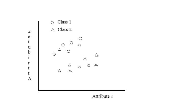
References Modifying one of the Machine Learning Algorithms kNN to Make it Independent of the Parameter k by Re-defining Neighbor
- Dutt S, Chandramouli S and Das AK. Machine Learning. Pearson India Education Services Pvt Ltd. Noida. 2020.
- Dhanabal S and Chandramathi Dr S. A Review of various k-Nearest Neighbor Query Processing Techniques. International Journal of Computer Applications 2011; Vol 31-No 7: 14-22.
- Uhlmann JK. Satisfying general proximity/similarity queries with metric trees. Information Processing Letters 1991; 40: 175-179.
- Liu T, Moore AW and Gray A. New Algorithms for Efficient High-Dimensional Nonparametric Classification. Journal of Machine Learning Research 2006; 7: 1135-1158
- Sproull RF. Refinements to Nearest Neighbor Searching in k-Dimensional Trees. Algorithmica 1991; 6:579-589.
- Li SZ, Chan KL and Wang C. Performance Evaluation of the NFL Method in Image Classification and Retrieval. IEEE Trans on Pattern Analysis and Machine Intelligence 2000; Vol 22-Issue 11.
- Zhou Y and Zhang C. Tunable Nearest Neighbor Class. Pattern Recognition 2007: 346-349 pp
- Liaw YC, Wu CM and Leou ML. Fast Exact k Nearest Neighbors Search using an Orthogonal Search Tree. Pattern Recognition 2010; Vol 43-Issue 6: 2351-2358.
- McNames J. Fast Nearest Neighbor Algorithm based on Principal Axis Search Tree. IEEE Trans on Pattern Analysis and Machine Intelligence 2001;Vol 23-Issue 9:964-976.
- Cover TM and Hart PE. Nearest Neighbor Pattern Classification. IEEE Trans Inform. Theory 1967; IT-13:21-27.
- Bailey T and Jain AK. A note on Distance weighted k-nearest neighbor rules. IEEE Trans Systems, Man Cybernatics 1978; 8:311-313.
- Kollios G, Gunopulos D and Tsotras VJ. Nearest Neighbor Queries in a Mobile Environment. Proceedings of the International Workshop on Spatio-Temporal Database Management 1999: 119-134 pp.
- Xia T and Zhang D. Continuous Reverse Nearest Neighbor Monitoring. Proceedings of the IEEE International Conference on Data Engineering 2006.
- Song Z and Roussopoulos N. K-nearest neighbor search for moving query point. Proceedings of the International Symposium on Spatial and Temporal Databases 2001: 79-96 pp.
