Monte Carlo numerical method in the problem of temperature stability analysis of electronic devices

approbation of the proposed methodology, the book authors give estimates of tolerances for several typical electrical circuits operating in a continuous and pulsed mode. The direct current electrical circuits are considered separately.

In a later paper [2], the calculating tolerance technique proposed in [1] was found to be a logical extension. The technique served to form the ED mechanical and electrical tolerance theory. The global mathematical model in this theory is the relative error equation of N ED output parameter:

^{A N} _ ^ ^д Ф i ^{( q}1,q 2,—, qn ) qi

N   i =1 .        ^d qi        ^ i ^{( q} 1, q 2,-, qn )

a i

A T ,

where ^^(q1, q2,.", qn)-------qi-------= B, - are the influence coefficients; ai - is the temperature aq;          Ф(q 1, q2,..., qn ) i coefficient of i-th ERE parameter; ∆T – is the difference between the ERE operating temperature and the ambient temperature; q1, q2, ..., qn – are ERE parameters; ϕ(q1, q2, ..., qn) – is the analytical dependence of N ED output parameter versus the ERE parameters.

Further development of the ED electric tolerance theory with reference to external and internal temperature influences was found in [3]. The author proposed an effective method for finding the B_i influence coefficients of the temperature error equation (1). The essence of the method is the use of experimental statistical planning in combination with regression analysis. In this case the global mathematical model is the regression equation:

kkk n = b о + Ё biqi + Ё bijqtq j + Ё buqi + -, i=1         i < ji where n – statistical evaluation of N ED output parameter; b0, bi, bij, bii – are the empirical coefficients of the regression equation.

The regression equation (2) makes it possible to estimate both linear and nonlinear interactions, depending on the experimental plan.

In the same paper [3] it was shown that for multiparameter ERE it is expedient to make a variation not by individual parameters but directly affect i -th element by temperature. If during statistical data processing we additionally normalize the regression coefficients in (2), then we obtain the temperature error equation:

n      nn

^A N ° ^UL = Z ^ A T i + EE aa

N out     t = 1 Ti    i = 1 j = 1

A T , A T ,

T i T j

+ -,

bi T 0

where ai =--is the influence coefficient of the i -th ERE; T 0 - is the nominal temperature (zero

A T -b о

A T, variation level); ∆T – is the temperature variation interval;    i – relative change in the ERE operating temperature.                                              Ti

The practical use of the temperature error equation (3) was demonstrated in [4, 5]. In particular, a regression analysis of the electronic circuit temperature stability was developed using computer circuit simulators, such as Cadence OrCAD and Spectrum Software MicroCAP.

Problem statement

According to the investigation results in [4, 5] it was established that the variation in the ERE operating temperature in the factor experiment is not always justified. There are electrical circuit classes in which N ED output parameter depends on one-parameter ERE (resistors, capacitors, inductors) mainly. Therefore, when carrying out a factor experiment it is sufficient to vary by one parameter for each such ERE. There is no need to take into account the temperature dependence of the interrelated (correlated) parameter complex within one ERE. Based on this, equation (1) takes the form:

A N _ n d^ q_; a n M ⁸ qi ф i ( qi ) ¹

A T .

The difference in the experiment planning course lies in another mechanism for obtaining a normalization factor:

Qi - q '. Q t - ± 1, qi   qi ₀

where ∆ q i = ( q i – q i 0 ) – is the variation interval (step) of i- th ERE parameter.

Applying the differentiation operation to (4) for each q_i factor, we obtain the temperature error equation according to [2]:

A N

N

k

^E A i ^a q t i = 1

k

+ ^E A y ^a q t ^a q j t <  u

+ U „> +-i = 1

A T ,

ь л   8n qi0

where A^ =

⁸ qi N о

– is the influence coefficient of linear terms;

A = a ² n qi о qj о ij = d qi d qj N 0

– is the mixed

second-order influence factor characterizing the ( i - j ) pair factor interaction on the output parameter;

л 2

, _ 52 N Я 20

iii = .2

d q_t ^N 0

– second-order influence coefficient.

In the final form, the temperature error equation for one-parameter ERE is:

n       nn

^ N out = ^ a i « i A T i + 2 E a j « i « j ^ T j + -,                     (7)

^N out     i = 1           i=1 j = 1

where ai – is the influence coefficient of i-th ERE thermal dependent parameter; bi – regression coefficient; α – maximum temperature coefficient value of the variable parameter; ∆T – working ii temperature changing of i-th ERE.

Thus, the problem of obtaining equation (7) can be reduced to the problem of efficiently finding the ai coefficients for electronic devices, at that temperature function of the N output parameter depends primarily on one-parameter electro radio elements.

Research theory part

The aim of the research is to improve the system design method of the thermostable ED with the numerical Monte Carlo method.

A common method of electrical circuits’ statistical analysis is the Monte Carlo method (the statistical test method) [6]. At the same time, the use of this method as applied to the study of the ED temperature stability generates two main problems:

• 1.    Search or synthesis of ERE mathematical models by criterion of adequacy of parameters’ temperature dependences to their real characteristics.

• 2.    Monte Carlo method realization according to the factor experiment scenario in order to justify minimization of the statistical test number.

The complexity of first problem solving is due to the fact that there are practically no adequate ERE mathematical models with parameters’ temperature dependences applied to the domestic element base. Separate attempts to create such models have been undertaken in [7, 8]. This article focuses on solving the second problem – the implementation of the numerical Monte Carlo method in the problem of analyzing the ED’s temperature stability.

The calculation block diagram using the Monte Carlo method (Fig. 1) includes the basic procedures:

• 1.    Random Q vector realization, i.e. generation of q_i component parameters’ random values in accordance with their distribution laws.

• 2.    A single-variant analysis of the electrical circuit with the obtained random Q vector realization.

• 3.    Calculation of the target V function’s value in order to establish the ED output parameter.

• 4.    Pre-set repetition of procedures No. 1, 2, 3, corresponding to the total test’s number.

• 5.    Statistical processing of the all tests’ results.

Approaches in the implementation of No. 1, 3, 5 procedures are specific for the numerical Monte Carlo method in the problem of analyzing the ED’s temperature stability. Let us consider this implementation in more detail.

It is known [9] that for single-parameter ERE (resistors, capacitors, inductors), the temperature coefficient characterizes reversible changes in the q parameter with a change in temperature. The parameter’s temperature coefficient (PTC) α – is its relative change with temperature change by 1 °С:

a

1 dq q=qdT ■

With a parameter’s linear temperature dependence, which is usually observed in a narrow range of ambient temperatures, the PTC calculates as:

_ q(T)-q(T) a q" q (To )(T-To) • where q(T), q(T0) – is the parameter’s value, respectively, at an increased (decreased) operating temperature T and at a normal temperature T0.

If the q ( T ) dependence is nonlinear, then the parameter’s temperature stability can be characterized by a relative change in the δ q parameter:

• _§    qTT )- q^T ⁰ ) .1_OO%.

^q     q TO^ )

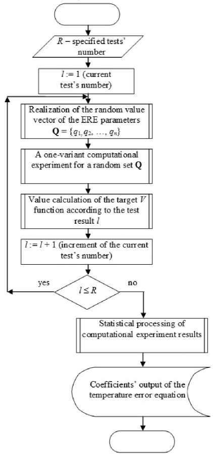
Fig. 1. Block diagram of the computational experiment realization for finding the coefficients of the temperature error equation

Let i -th ERE of the electrical circuit have a functional q ij parameters’ set ( Set i vector):

Set i = { q i 1 , q i 2 , q i 3 , …}.

From the position of the temperature stability investigation of i -th ERE, each functional parameter is a temperature function. Consequently, Set i is also a vector function versus temperature:

Set i ( T ) = { q i 1 ( T ), q i 2 ( T ), q i 3 ( T ), …}.

In the special case of one-parameter ERE (elements with one pronounced functional parameter), the vector function degenerates into a one parameter’s function versus temperature:

Set i ( T ) = { q i ( T )} → q i ( T ). (8)

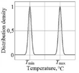
The T temperature, inherent in i -th one-parameter ERE under both external and internal thermal effects, is probability value. Suppose that the probability T value for i -th ERE is subject to the normal distribution law:

f(T )=  lp_(TzT)2

o \2n         2o2

where f ( T ) – is the probability density function of the random T value; T 0 – is the normal temperature; σ – is the standard deviation of the random T value.

Define a certain range of operating temperatures for i -th ERE: [Tmin, Tmax]. According to the factor experiment scenario [5], the operating T temperature of i -th ERE can be equiprobably near the point T 0min and T 0max estimates. Then the sum of the probability density functions of a random T value is a bimodal distribution’s density function:

bi(T ) =

^f T min ) + f (T max)

norm

1 normFlK

<-----exp

^ min

—

^T min ^T 0min

2 a²-min

1         (T max- T 0max)2

exp         ₂

^a max L ^{2 a} max .

where norm – is the normalizing coefficient; T _min and T _max – random values of operating temperatures at the given range’s boundaries; σ min and σ max – are the corresponding T min and T max standard deviations.

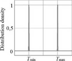
Obviously, the computational factor experiment, in contrast to the real experiment, allows us to specify the variation levels’ values with high accuracy in each experiment realization. Consequently, under the conditions of the computational factorial experiment: (σ ≈ σ ) → 0. This effect is m n max graphically shown in Fig. 2. The bimodal distribution’s density function can be written more simply:

bi ( T ) =       1       l exp T- ( T min - TO ) 2 1 ₊ exp T- ( T max" T O') 2 1^ .

norm- □ V2 n[   [      2 ct ²   ]     [      2 a ²     ]

The limiting case, when σ = 0, allows us to introduce the discrete random T value’s notion, i.e. operating temperature of i -th ERE, taking only the T _0min and T _0max values. The discrete random T value is determined by the Bi ( T ) distribution function analytically:

а

IcmpCTaturc.X

b

Fig. 2. The bimodal distribution’s density function of the random T value: а – ( σ ≠ 0) case, b – ( σ → 0) case

0 e ( oo ; T min ] ;

Bi ( t ) = ■

0,5 ^{e ( t} min ; ^T max ] ;

¹ e⁽ T max i +oo ) .

The graphical form of the Bi ( T ) distribution function is shown in Fig. 3.

As a result, for i -th ERE function (8), the definition domain consists of only two values:

q i ( T ) = q i

T imin . T max

The q i ( T ) function is, in its turn, one of the parameters for the ED’s relative error equation (4).

Therefore, as applied to equation (4), the admissible parameters for i -th ERE are:

Q i =

„ min qi max

I qi    J

The computational experiment factors’ area is the set of all q_i :

( min 1

^ max

Q = ^

min

max q ₂

Qn =

min q n

. qm^ax

where n – is the factor number, i.e. the one-parameter ERE number are varied in the experiment.

Under the conditions of realization of the computational factor experiment, a V vector will be obtained. The V vector’s element is represented by the θ _i function of the ED’s one-variant test, which contains a unique (non-repetitive) q i value’s combination:

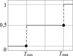
Temperature, °C

Fig. 3. The distribution function of a discrete random T value min min min

V1 = ⁰ 1 ^{( Q} b Q 2,-, Qn ) =⁰ 1 V1   , q 2 ,-, qn ) ;

V = к = 0 2 ( Q l, Q 2,..., Qn ) = 0 2 ( q max, q 2™™,-, q T) ;

max max max

Vm = 0m(Ql, Q2,—,Qn)=0m(q1   ,q2 ,—,qn ) , where m = 2n.

Statistical processing of the computational experiment is aimed at finding the coefficients’ regression. We introduce an auxiliary K matrix with m × ( n +1) dimension containing the code values of variable factors’ levels:

1 — 1 ... — 1

K =

1      1 ... 1

The zero matrix column (leftmost) contains unit values and is intended to calculate the free term of the regression equation:

_ V^T K ^{< 0 >} b 0 =

m

The remaining columns of the K matrix (from 1 to n ) serve to calculate the coefficients’ regression of the corresponding factor:

, VT K<1>     , b1 =----------; ^; bn =

m

VTK< n >

m

The factors’ non-linear interaction in the computational experiment can be taken into account by adding columns with the code realization of the q_iq_j , q_iq_jq_k , … factors. It is obvious that the nonlinear interaction study will lead to an increase in the dimension of the K matrix to:

m × (n+1+p), where p – is the number of factors’ nonlinear interactions.

To find the temperature error equation (7), it is necessary to recalculate the b i coefficients’ regression in the a_i influence coefficients of the thermally dependent parameter of i -th ERE:

b q ⁰

a; = i

Aqi • bo ’ where qi0 – the zero level of the variable parameter of i-th ERE; ∆qi – the variation interval of the qi0 value.

Research experiment part

The object of experimental research is the electric circuit of the harmonic oscillations’ generator with the Wien bridge (Fig. 4). The generator uses VD1 and VD2 zener diodes to limit the output signal.

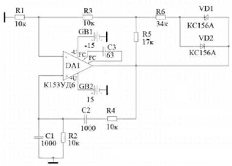
Fig. 4. Wien bridge circuit

The circuit is characterized by a harmonic distortion coefficient in the range 1 ... 5 % [10]. To generate oscillations in the generator, the Barkhausen criterion must be complied: the phase shift of 180 ° occurs in the feedback loop; the total gain in the loop is not less than one.

In the circiut R2 = R4 = R and C1 = C2 = C. Consequently, the theoretical quasi-resonance frequency is:

f =   ¹

2 π RC

= 15923 Hz. 2 π 10⁴ 10 ⁹

Using the frequency correction circuit (DA1, C3), the oscillation frequency is reduced to 10 kHz. The aim of the research experiment part is to find the temperature error equation (7) for a generator

Δf with a Wien bridge. The ED’s output parameter is the relative instability    of the generation frequency.

f

One-parameter ERE, most influencing the output parameter, are: C1, C2, C3, R2, R4.

The generator element base with the Wien bridge consists of four ERE types and four corresponding SPICE models (Table 1). For carrying out the computational experiment, the following ERE types are specified:

• -    for C1, C2 apply

ОСК10-17В-М47-1нФ±5 % В ОЖ0.460.107 ТУ;

• -    for C3 apply

ОСК10-17В-М47-63пФ±5 % В ОЖ0.460.107 ТУ;

• -    for R2, R4 apply

ОСМ Р1-8МП-0,5-10кОм±0,1 %-0,5-М-А-ОЖ0.467.164 ТУ.

According to [11, 12], the resistance temperature coefficient of the resistors’ types is α R = ±100·10^-6 C^-1; the capacitance temperature coefficient of the capacitors’ types is α C = -47·10^-6 C^-1.

– 521 –

Table 1. SPICE model list used in the Wien bridge modeling

No.	SPICE model name	Origin source
1	Thin film chip resistor Р1-8МП	“SPICE-model development of Russian-made electronic component base’s library” report
2	Chip capacitor for surface mounting К10-17В	“SPICE-model development of Russian-made electronic component base’s library” report
3	Silicon zener КС156А	r-diod.lib library, part of the Spectrum Sofware MicroCAP simulator (Russian localized version) [13]
4	Medium accuracy operational amplifier К153УД6	r-opamp2.lib library part of the Spectrum Sofware MicroCAP simulator (Russian localized version) [13]

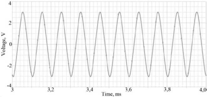
Fig. 5. Oscillation generation in the nominal mode ( f = 10 kHz, U m = 3V)

In the nominal mode (no parameters’ variation), the simulation of the generator’s circuit with the Wien bridge was carried out in the OrCAD PSpice simulator [14]. The result were harmonic oscillations of f = 10 kHz frequency and U_m = 3V amplitude (Fig. 5).

To accurately fix the f and U m numerical values the PSpice Probe graphic postprocessor two target functions are formed:

1/Period(V(DA1:OUT));

Max(V(DA1:OUT)), where Period – is the target function template for finding the oscillation period [14]; Max – is the target function template for finding the oscillation amplitude [14]; V (DA1: OUT) – is the target functions’ argument, denoting the potential at the OUT output of the DA1 operational amplifier (and the whole circuit).

The main characteristics of the computational experiment plan are given in Tables 2, 3, 4. Note that the capacitor types used have a linear capacitance temperature coefficient (M47) over the entire operating temperature range [12]. The resistor type has a non-linear resistance temperature coefficient (M) [11], however, due to the small temperature range in the computational experiment (±10 °C), it is permissible to use a linear dependence. Thus, during computational experiment planning the parameter’s temperature dependence was used for all variable ERE:

N ( T ) = N 0 (1 ± TCN ·∆ T ), where N 0 – is the nominal parameter value; TCN – is the parameter’s temperature coefficient; ∆ T = ±10 °C – variation interval temperature.

Based on the results of the computational experiment planning, the relative deviation (DEV) of the ERE’s scale parameter is found necessary for the Monte Carlo statistical tests (the penultimate column):

.MODEL K10-17 CAP (C=1 DEV=0.047 %);

.MODEL R1-8 RES (R=1 DEV=0.1 %).

Table 2. Variation levels for C1, C2 (x1, x2 factors)

	Capacitor operating temperature T , °C	Absolute capacity value С ABS , nF	Temperature variation interval ∆ Т , °С	Capacity absolute deviation ∆ С , nF	Capacity relative deviation -С— -100% С ABS	C scale factor deviation for the SPICE model
Top level	37	1,00047	+10	+0,00047	+0,047	1,00047
Zero level	27	1	0	0	0	1
Bottom level	17	0,99953	-10	-0,00047	-0,047	0,99953

Table 3. Variation levels for C3 (x3 factor)

	Capacitor operating temperature T , °C	Absolute capacity value С ABS, nF ABS	Temperature variation interval ∆ Т , °С	Capacity absolute deviation ∆ С , nF	Capacity relative deviation -С— -100% С ABS	C scale factor deviation for the SPICE model
Top level	37	63,02961	+10	+0,02961	+0,047	1,00047
Zero level	27	63	0	0	0	1
Bottom level	17	62,97039	-10	-0,02961	-0,047	0,99953

Table 4. Variation levels for R2, R4 (x4, x5 factor)

	Resistor operating temperature T , °C	Absolute resistance value R ABS , Ohm	Temperature variation interval ∆ Т , °С	Resistance absolute deviation ∆ R , Ohm	Resistance relative deviation -R- -100% R АBS	R scale factor deviation for the SPICE model
Top level	37	10 010	+10	+10	+0,1	1,001
Zero level	— 27	10 000	— 0	0	0	1
Bottom level	17	9 990	-10	-10	-0,1	0,999

Multivariate analysis of the electrical circuit (Fig. 4) using the Monte Carlo method is carried out in the OrCAD PSpice simulator. The circuit simulation parameters (Fig. 6, 7) are:

• -    run to time: ∆ t = 4 ms;

• -    start saving data after: t beg = 3 ms;

• -    skip the direct current analysis;

• -    output variable – output voltage of the op-amp: U OUT = V ( DA 1: OUT );

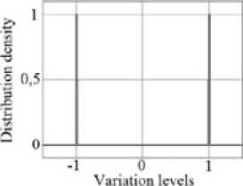
• -    test number by the Monte Carlo method: MC = 100;

• -    name of the random variables’ distribution law: BiModal ;

• -    random number seed: No = 1;

• -    coordinates of the normalized bimodal distribution law: (–1,1) (–0.99,1) (-1,1) (-0.99,1) (-0.99,0) (0.99,0) (0.99,1) (1,1).

The result of the multivariate analysis is the family of harmonic oscillations originally. However, such a graphical representation is inconvenient for perception and quantitative analysis. The noted deficiency is easily eliminated. The functionality of the PSpice Probe graphical postprocessor makes it possible to present the values of the target function (12) in a table form in each of the statistical tests (Fig. 8).

b

» Hixi»C*to P Frw>l^F

Г Wt» O^¥*^t4e [V1DA1 ОМП Месте Cebopbcni

Hwbwd»X*     "LU

Ui* <4dib/w.     ^H^d 5 OulihUrcu |

H-ydyri fonbe» i«d *      |1, ЗУвЛ iieve Me Voiti 41     "Xi I        ' w

c

Rsistolne          [4m       seconds (T$TOP1

Sial satay dale a*» | An        sKusids

Tiimwr* nchtini

Ммямл aep urn |o In wcndt

P GM> farAd brant Ым por* c^cUMen ^JPOP)

a

Fig. 6. Modeling parameters: a – time domain analysis parameters, b – Monte Carlo analysis parameters, c – bi-modal distribution parameters

Fig. 7. The normalized density of the bimodal distribution

Fig. 8. Table of Monte Carlo test results

Each of the statistical test’s results (Fig. 8) should be compared with a specific combination of variable factors. The essence of the comparison lies in the comparative analysis of the output text file (Fig. 9, a) generated by OrCAD PSpice, and the information presented in the implementation matrix of the computational experiment (Fig. 9, b, c).

For example, in a text file, a fragment with test No. 87 was found, with the following combination of ERE parameters:

С1 = 9,9953Е-01; С2 = 9,9953Е-01; С3 = 9,9953Е-01;

R2 = 9,9900E-01; R4 = 9,9900E-01.

According to Table 2, 3, 4 it is easy to establish that the code values of the factor combination looks like:

С1 = -1; С2 = -1; С3 = -1; R2 = -1; R4 = -1.

Therefore, the test No. 87 and the target function value f = 10,02792 kHz, found from the table in Fig. 8, will correspond to the combination (-1 -1 -1 -1 -1) in the computational experiment implementation matrix.

The orthogonality of the implementation matrix’s columns (Fig. 9, c) allows us to determine the regression coefficients according to (9) and (10):

b0 = 10,014·10³; b1 = 0,00146·10³ (С1); b2 = –0,00587·10³ (С2);

b3 = –0,00046·10³ (С3); b4 = –0,01248·10³ (R2); b5 = 0,00312·10³ (R4).

Consequently, the linear polynomial has the form:

f = (10,014+0,00146q1– 0,00587q2 –0,00046q3 –0,01248q4 +0,00312q5)·10³.   (12)

Using the obtained linear polynomial (12), we calculate the theoretical value of the output f_Т parameter in each experiment, and then find the sum of the difference squares between the experimental and theoretical values of the output parameter. The total sum of difference squares of values for a linear polynomial is ∆f² = 4,96·10^-8·10³. Taking into account the small value of ∆f², we can consider (12) to be an adequate regression model.

According to (11), the coefficients of the temperature error equation are determined:

a1 = 0,311 (С1); a2 = –1,247 (С2);

a3 = –0,097 (С3); a4 = –1,247 (R2); a5 = 0,312 (R4).

The temperature error equation in accordance with (7) will be:

^Δ_f^f=1,46 10^-5ΔT_C1-5,86 10^-5ΔT_C2-4,55 10^-6ΔT_C3

-1,25 10^-4ΔT_R2+3,12 10^-5ΔT_R4.

Research results

Analysis (13) allows us to state:

• –    the temperature error of the generation frequency mainly depends on the temperature instability of the four ERE: C1 and C2capacitors, R2 and R4 resistors;

• –    the linear polynomial (12) is recognized as an adequate regression model of the investigated process;

• –    to ensure a given temperature stability of the generator, three solutions are possible: the use of highly stable C1, C2, C3, R2, R4; partial temperature compensation of C1-C2 and R2-R4 pairs; thermostating R4.

Conclusions

• 1.    A modification of the numerical Monte Carlo method for analyzing the temperature stability of electronic circuits is proposed.

• 2.    The problem of finding the influence coefficients of the temperature error equation for the one-parameter ERE’s case was solved.

• 3.    The obtained temperature error equation of the generator with the Wien bridge (13) allows quantitatively and qualitatively to formulate the requirements for ensuring a given temperature stability of the device both at the stage of circuitry and at the stage of topological design.