МРТ-идентификация и классификация опухолей головного мозга с использованием DWT, PCA и машины опорных векторов ядра

DOI:

An Image in image processing symbolizes the under-standing that object data was also processed to produce an image. Clinical personnel are now better equipped to pro-vide patients with healthcare thanks to the recent use of technology and electronic healthcare systems in the medical industry [1]. In order to identify the issue of segmenting aberrant and normal tissues from MR images, this study employs the gray-level co-occurrence matrix (GLCM) for feature extraction and probabilistic neural network (PNN) classification. Brain tumors are caused by the uncontrolled growth of aberrant, malignant tissue. Both benign and malignant brain tumors are possible. The benign tissue has cancer cells that are unrelated to the tumor and are physically equivalent. The malignant tumor contains active cancer cells that move across regions and has irregularly shaped features.

Malignant tumors are categorized on the scales from Grade I to Grade IV, which are utilized in the grading system. Tumors of grades I and II are of lesser grade, whereas those of grades III and IV are of greater grade [7]. At any age, brain tumors can affect people. It might not affect everyone in the same way. The complexity of the human brain makes it challenging to diagnose the tumor region there.

Malignant grade III and IV tumors are rapidly developing. It damages the proper brain cells, has the potential to spread to all other sections of the central nervous system (CNS), and can be dangerous if left untreated [9]. The early detection and categorization of such brain tumors is thus a critical concern in medical science. It enables a physician to monitor and follow the occurrence and progression of malignant cell regions at various stages by enhancing the most recent imaging techniques, allowing them to make reliable diagnoses by scanning these pictures.

The biggest problem was finding brain cancers in time for proper therapy. Based on these factors, the best radiation, surgery, or chemotherapy therapy can be decided. As an outcome, it's also obvious that early diagnosis of a tumor can considerably boost a tumor-infected patient's chances of survival [26]. Using imaging methods, segmentation is used to evaluate the part of the tumor that is affected. It is the process of dividing an object into component parts that share similar properties such as color, texture, contrast, and borders.

Human brain tumors are among the primary causes of mortality. It is clear that if the tumor is recognized early and detected effectively, the chances of survival may in-crease. Invasive approaches include the usual technical procedures for identifying and classifying benign (noncancer) and malignant (cancer) brain tumors, including biopsies, lumbar punctures, and movements of the spinal tap.

A computer-assisted diagnostic algorithm was developed to replace traditional invasive devices and time-consuming techniques in order to increase brain tumor di-agnostic accuracy and classification. This article de-scribes a high-quality tumor classification approach in which individual magnetic resonance (MR) pixels are categorized as common genius tumors, non-cancerous tumor letters, and malignant tumor letters. There are three phases in the proposed method: (1) wavelet decomposition, (2) texture extraction, and (3) classification. The MR image was initially decomposed into unique steps with defined approximation coefficients using discrete wavelet processing with Daubechies' wavelet (db4), after which structural data such as forces were acquired. The suggested technique has been applied to real MR images, with a classification accuracy of over 98% utilizing probabilistic neural networks.

LITERATURE REVIEW

Image Acquisition

Pre-Processing

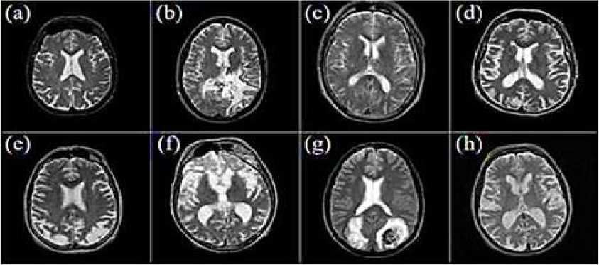
Figure 1. MRI brain picture: (a) natural brain; (b) Glioma; (c) Meningioma; (d) Alzheimer's illness; (e) Alzheimer's illness with visual agnosia; (f) Pick's disease; (g) Sarcoma; (h) Huntington's illness.

Five different levels are created by dividing the images of the MRI by the identical coefficients of the LL and HL bands. Such sub-bands have been attained from the disarranged wavelet; GLCM has been used to extract quantitative textural features such as strength, corelation, entropy, and homogeneity [3]. Filtering and de-noising pictures (shown in Fig. 2) are the initial stages of image pre-processing. Certain recovery approaches are used to eliminate generated noise that might enter a picture during capture, transfer, or compression. [2].

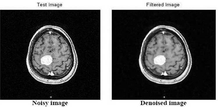
Figure 2. Example of noisy image and reduction of noise.

Segmentation of Image

Image segmentation is the procedure of splitting an image into distinct segments, each with comparable features in Figure 3. depicts the many types of image segmentation [1, 24].

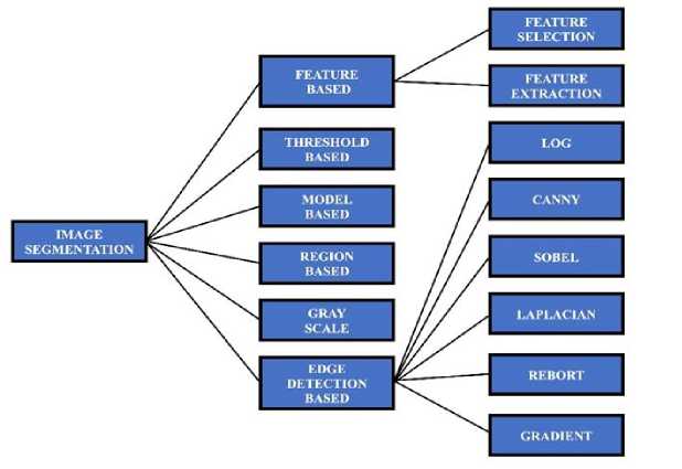
Figure 3. Image segmentation types.

Feature Extraction

Five different levels are created by dividing the images of the MRI by the identical coefficients of the LL and HL bands. Such sub-bands have been attained from the disarranged wavelet; The GLCM has been used to extract quantitative textural characteristics such as strength, co-relation, entropy, and uniformity [10]. Filtering and de-noising pictures are the initial stages of image pre-processing. De-noising is the technique of eliminating artificial noise from a picture before capturing, transmission, or compression utilizing specialized recovery algorithms [2]. Picture segmentation is the process of dividing an image into distinct segments, each with comparable features. As seen in figure 3, there are several forms of image segmentation [11, 17]. Feature extraction is the process of retrieving statistical data from an image that resembles color characteristics, texture, shape, and contrast [12]. We employed the discrete wavelet transform (DWT) to extract wavelet coefficients and the GLCM to obtain applied math features. Feature extraction is the process of choosing subsets from the set of variables that demonstrate the behavior of the entire set. choosing the helpful variables and discarding the inapplicable ones.

Pictures 1 to 8 display various sub-band levels up to the decomposition stage of the 5th wavelet. As an input vector, the extracted form was used to train and evaluate the output of the PNN types. The characteristics of the statistical field are shown in Table 1 [3].

Picture	Contrast	Correlation	Energy	Homogeneity	Entropy
Pic1	0.386541	0.0805	0.81568	0.900	2.3224
Pic2	0.360122	0.1725	0.81607	0.9474	0.2244
Pic3	0.265017	0.1248	0.77808	0.9383	2.8746
Pic4	0.315628	0.0928	0.79636	0.9404	2.6739
Pic5	0.365406	0.1353	0.80855	0.9447	2.5116
Pic6	0.285873	0.1143	0.75812	0.9315	2.8806
Pic7	0.299221	0.1129	0.78455	0.9387	2.9101
Pic8	0.267241	0.1246	0.77884	0.9367	2.9114

Image Classification

Image classification is the extraction of data classes from bitmap image having numerous bands. The real three types of classification are per pixel, per subpixel, and object.

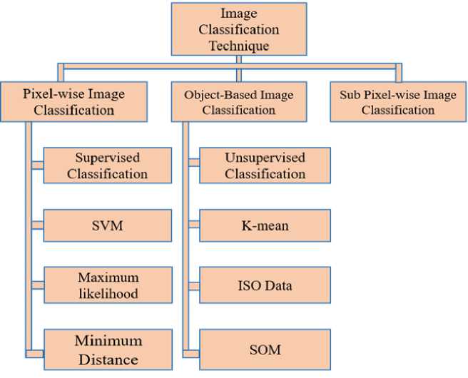
Figure 4. Different types of techniques for image recognition.

This study concentrated on pixel-scale image categorization [4], which is classified into three categories.: The two most common approaches are supervised classifiers (manual) and unsupervised classifiers [5, 6], (calculated by the software), but analytical object-based images are rare and the most recent technique, as mentioned above, and the analysis is fed with high-resolution images. Figure 4 depicts the various types of object classification from different points of view.

METHODOLOGY

The suggested method for the identification of brain tumors involves five major steps:

• •    Extraction of features using DWT

• •    Extraction of textures using GLCM

• •   Selection of features using PCA

• •    Detection of tumors and K-means structural analysis

• •   Using PNN-RBF Network identification

  Extraction of features using DWT

  

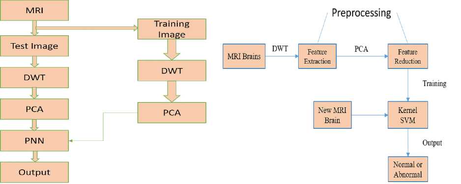
  Figure 5. Six-stage image reference block diagram to output.

  
  

w ^ ^a, b) = f -° _m f(x) * ^_ab(t)dx ,

where ^ a,b⁽ t ⁾ =^j

As a function vector, the proposed system makes use of the coefficients of the Discrete Wavelet Transform (DWT). The wavelet is a powerful mathematical tool for extracting facets and determining the wave coefficient from images; where employed MR. In Figure 5, Six-stage image reference block diagram to output. Wavelets are twisted as well as resized variations of constant-moment wavelets that have localized basic properties. Wavelets have the primary advantage of imparting localized frequency records about a signed variable, which is especially useful for ranking. A quintessential review of wavelet decomposition is delivered as below: (t) is a continuous wavelet transformation of the ax(t) signal with a squareintegrable characteristic, unlike a real-value wavelet. An indispensable evaluation of wavelet decomposition is delivered as below: A continuous wavelet transformation of an ax (t) signal, a squareintegrable feature comparative to a real-value wavelet (t), is defined as:

WT_x ( _n ) = {

d j, _k = Е(х(п)й * j (n - 2 j k)) d j, _k = ^(x⁽n⁾g *j⁽n - 2jk⁾)‘

Wavelets a and b are defined by translation and dilation from the mother's wavelet, wavelet, dilation factor, and b translation parameter (both of which are real, high-quality numbers). Under some mild assumptions, the base wave-let responds to the limit of having zero meaning. The equation can be debunked by means of limiting a and b to a discrete lattice, which gives the discrete wavelet [7].

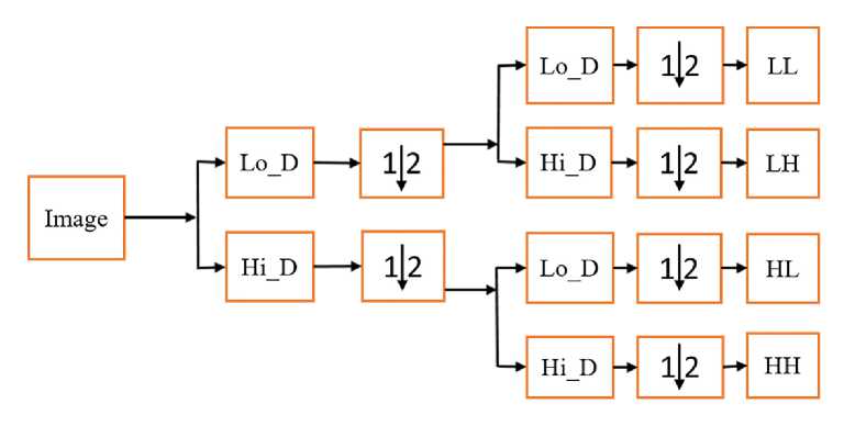
Figure 6. DWT Schematically.

The technique that divides information into different wavelength elements and analyzes these elements with a precision proportional to their size is known as DWT:

Ho_D – High Pass Filter, Lo_D – Low Pass Filter.

The Daubechies wavelet is thought to have the best quality for image utility based on literature analysis, and among the other wavelets, LH's overall performance was once better than the HL sub-band characteristics, shown in Figure 6. The qualities were then extracted from the DWT sub bands LH and HL, and a five-level decomposition of the Daubechies wavelet usage was determined in this approach.

Extraction of textures using GLCMs

Examination of the texture makes it easy to distinguish between regular and anomalous tissue. It even contrasts malignant tissue to regular tissue, which can be un-der the person’s experience level. Texture evaluation is one of the uses of computer-assisted pathology as a supplement to strategies for biopsy. This technique calculates a specific gray level frequency in a random photograph region and does not take the correlations between pixels into consideration. Using this strategy, the frequency is computed at a specific gray level in a random image region. It no longer takes into account pixel associations. The chance of detecting a pair of grey ranges at very vast distances and with intention throughout a full body is the base of statistical texture analysis in second-order texture recording. Using the GLCM additionally acknowledged as the Gray Level Spatial Dependence Matrix (GLSDM), statistical aspects of the MR snapshots are obtained. Haralick's GLCM is a statistical technique for explaining the connection between pixels of a particular gray level. GLCM is a two-dimensional histogram where (I, j) is the variable and the prevalence frequency is (I, j). It is an interval feature with d = 1, perspective 45, ninety, and one hundred thirty-five, and greyscales I and j calculate the frequency with which a pixel has an intensity I that is about to positively outstrip and an orientation in relation to another pixel j. The gray degree co-occurrence matrix and the statistical field elements such as contrast, interrelationship, and electricity are formed in this way. Homogeneity and entropy were obtained from the first five wavelet decomposition degrees of the LH and HL sub-bands [3].

Equation Selection of features using PCA

The element-component analysis is the best way to do dimension reduction. In PCA, the linear data seeks the lower dimensional in such a way that the replicated data variance due to a set of data is preserved. Limiting the feature vector calculated from waves based on a combined feature vector component analysis using a feature reduction system to a variable chosen by the PCA will result in an effective classification algorithm using a monitoring method, shown in Figure 7.

The purpose of PCA is to diminish the complexity of the wavelet coefficient. It operates under a classification that is much more descriptive and precise.

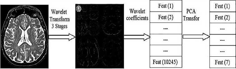
Image (256*256)

Figure 7. Block diagram for the extraction and reduction of the feature used.

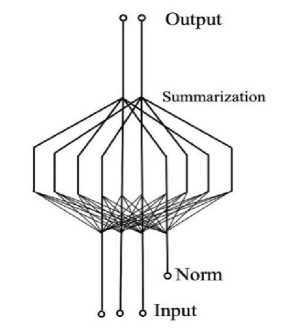
Using the Probabilistic Neural Network (PNN) Classification

It is a neural feed-forward network derived from a Bayesian network and Kernel Fisher's discriminatory analysis statistical algorithm [19, 25, 21, 22]. D.F. implements it. Specht's operations were founded in early 1990s on a four-tiered, multilayered, feed-forward net-work based on a PNN: in layer: 1. Input, 2. Pattern /Summation, 3. Output, 4. Hidden.

Probabilistic Neural Network Architecture: PNN layers: PNN is regularly used in problems with classification. When an entry is present, the very first layer calculates the gap between the entry vector and the entry vectors of the layers. Probabilistic Neural Network (PNN) architecture used to evaluate this research for MRI image identification and classifications, the architecture shown in Figure 8. It generates a vector in which the factors indicate how close the center is to the center of the learning [7, 19]. Level 2 adds up the benefits of every in-put class and generates its internet output like a probability vector. Then, a real switch characteristic on 2D layer output selects the greatest of these chances and generates a 1 for that type and a 0 (obstructive identity).

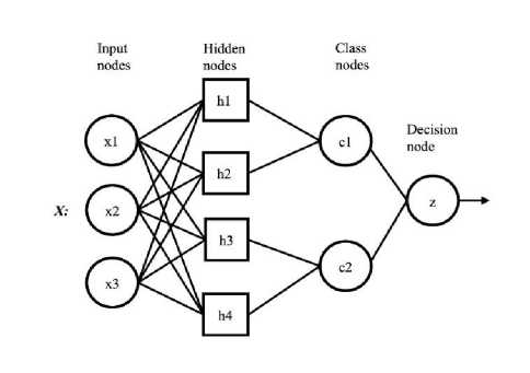
Figure 8. Architecture of PNN.

EXPERIMENTAL RESULT AND DISCUSSION

The tests were performed with a 5.0GHz processor and 32 GB of RAM on the Intel i7 platform running Windows 10. Using the wavelet toolbox to develop the algorithm, Matlab's 2018 bio statistical toolbox (Mathworks°c) was used. Install a free SVM toolbox, expand the SVM kernel, and use the classification of the MR brain picture. On any software platform where Matlab is available, the pro-grams can be run or checked. We tested four SVMs using the most recent Di® kernels. The SVM using a linear kernel is called KSVM [14, 16].

Table 2. Confusion matrix of our DWT+ PCA+KSVM method (Kernel pick out LIN, HPOL,

IPOL).

Approach from existing study	Accuracy(%)
SOM+DWT	95
SVM+ DWT with linear kernel	96
SVM+ DWT with RBF based kernel	98
PCA+KNN+ DWT	98
PCA+ANN+ DWT	97
PCA+ACPSO+FNN+ DWT	98.75
Approach from this study	Accuracy(%)
PCA+KSVM+ DWT (LIN)	95.38%
PCA+KSVM+ DWT (HPOL)	96.53%
PCA+KSVM+ DWT (IPOL)	98.88%
PCA+KSVM+ DWT (GRB)	99.61%

Table 3. A comparison of the classification accuracy of eight different algorithms using the same MRI dataset and the same number of images.

Parameter	Base	Accuracy
LIN	NORMAL [O]	ABNORMAL [0]
Normal (T)	18	3
Abnormal	5	230
HpoL	NORMAL[O]	ABNORMAL [O]
Normal (T)	19	1
Abnormal (T	4	232

Современные инновации, системы и технологии // (сс) ® 2024; 4(1) Modern Innovations, Systems and Technologies

IPOL	NORMAL [O]	ABNORMAL [O]
Normal (T)	18	2
Abnormal (T	1	239
GRB	NORMAL [O]	ABNORMAL [O]
Normal (T)	20	0
Abnormal (T)	1	239

The results reveal that the proposed DWT+PCA+KSVM technique generates outstanding results both at the training and validation datasets. S um up the overall classification performance of the LIN, HPOL, IPOL, and GRB kernels in table 2. The GRB kernel SVM architecture which provides the best the kernel's com-pared to others three SVMs kernels [15].

Furthermore, we evaluated our technique to six successful techniques disclosed in the current papers employing the same MRI datasets and image count. Table 2 dis-plays the results of the analysis. It demonstrates that our suggested DWT+PCA+KSVM system with the GRB kernel outperforms the other 8 approaches, obtaining the greatest classification performance at 99.38 percent. The next technique is the DWT+PCA+ACPSO+FNN method, which has a 98.75 percent accuracy. The fifth is our suggested DWT+PCA+KSVM IPOL kernel, which has a classification accuracy of 98.12% [13, 23].

Table 4. GLCM of LL and HL sub bands of tested images & statistic field.
Pictures	Psnr	Mse	Area of Picture in pixel	Area of the tumor region
Pic1	13.011	5.121	38,240	7598
Pic2	12.82	2.116	66,824	9774
Pic3	13.12	6.068	49,508	7532
Pic4	14.86	5.77	49,388	8956
Pic5	12.79	4.84	23,964	4465
Pic6	12.82	6.79	49,429	3598
Pic7	12.99	5.92	49,298	5979
Pic8	13.004	6.35	34,040	12,932

Table 5. The declaration of the region and the success of the evaluation of tumors extraction location of trained image.

Pictures	Con	Cor	Ene	Hom	Ent
Pic1	0.2755	0.106333	0.72044	0.92139	3.3209
Pic2	0.2611	0.129665	0.76435	0.93428	3.3830
Pic3	0.2611	0.129665	0.76435	0.93428	3.2821
Pic4	0.2929	0.156369	0.82164	0.94967	2.7610
Pic5	0.2469	0.07749	0.74696	0.92848	3.3895
Pic6	0.2416	0.177739	0.77415	0.9373	2.5186
Pic7	0.2611	0.12966	0.76435	0.93428	3.2820
Pic8	0.3053	0.09188	0.7674	0.9326	2.9181

The training data set objects were those for which the extracted features were classified using the PNN algorithm, whereas the test set was not trained and just statistical and textual characteristics were extracted. The comparison of the category of training and tested datasets using probabilistic neural networks, shown in Figure 9. The correctness of the qualifying and verified image was determined by classifying malignant cells as either normal or abnormal [20, 21]. Figure 10 depicts the results of the identification of malignant and non-malignant tumor tissues.

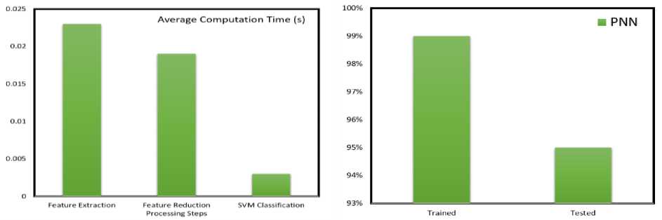
Figure 9. The categorization of training and tested datasets using probabilistic neural networks is compared.

The efficacy of an acceptable classification proportion to the actual number of form is referred to as prediction performance or "correct level" [19]. The brain tumor classification procedure was applied to a variety of both nor-mal and abnormal MR images, and the performance of the PNN predictor was modified using the equation shown be-low:

Calculation time is also an important factor in classifier evaluation. Since the SVM parameters stayed the same after training, the SVM training time was not taken into account.

All 260 images were fed into the classifier. The time spent at each stage of the DI® event was plotted in Fig. 10, along with the associated computation time, average value, and reported computation time.

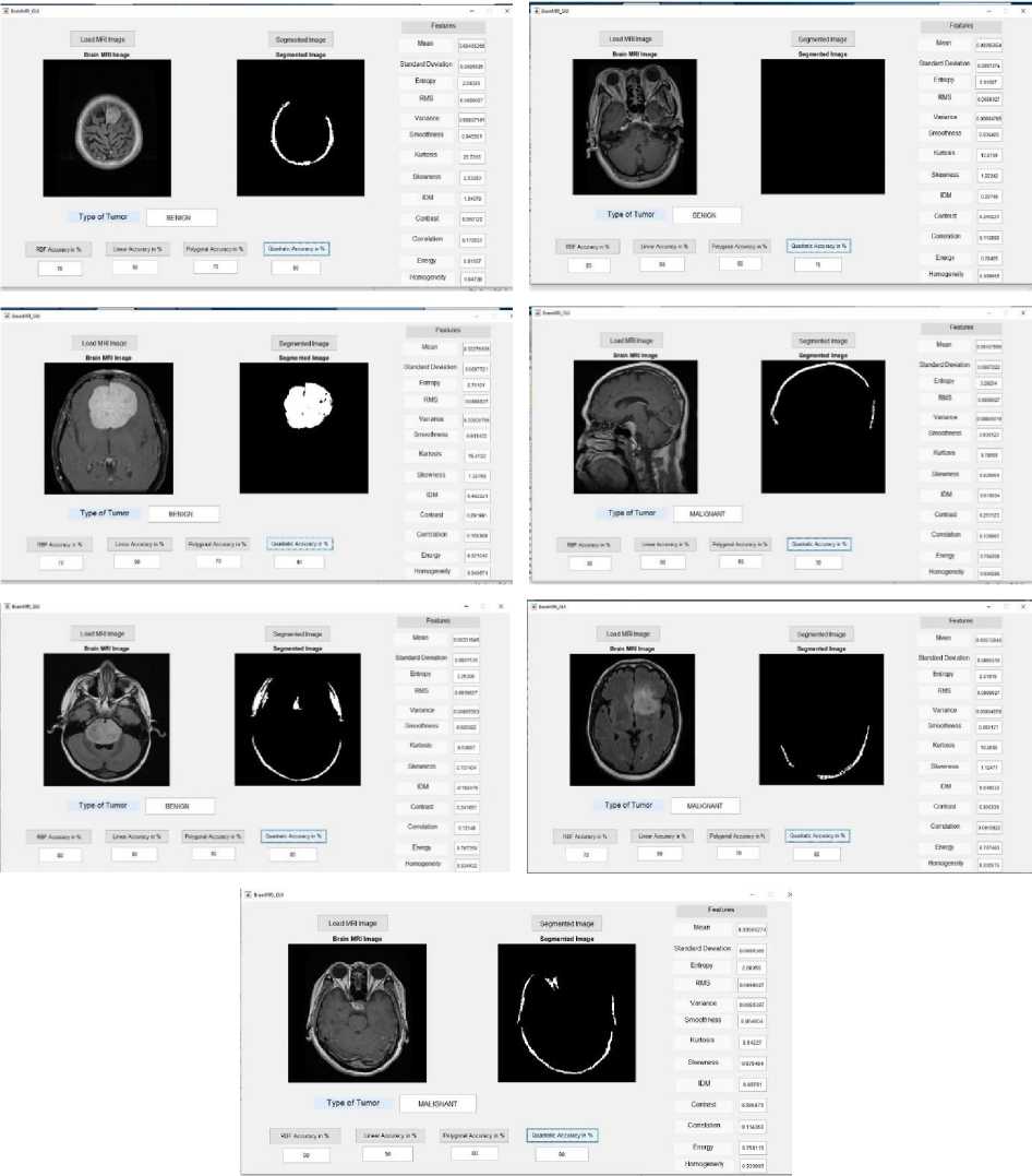
Figure 10. Segmentation and Classifying of Tumor.

In this lesson, we also created a brand-new DWT + PCA + KSVM technique to differentiate between authentic and artificial brain MRIs. We selected four different kernels for the LIN, HPOL, IPOL, and GRB [8, 24]. The study's findings show that the GRB kernel SVM outperformed the HPOL, IPOL, and GRB kernels as well as other well-known methods, achieving a classification performance of 99.38% on the 260 images from MR. For the public review and improvement of research This research papers have two preprints [26, 27].

CONCLUSION

In this research, we used brain MRI images separated between healthy (unaffected) brain tissue and aberrant (infected) tumor tissue. Preprocessing is used to eliminate noise from images and smoothing them out. This also helps to increase the signal-to-noise ratio. As a result, we applied a discrete wavelet transformation, which breaks down the image and extracts the features from the GLCM, which was detected using structural procedures. PNN could be a classifier used to perceive tumors in brain MRI images. According to research findings, diagnosing a brain tumor yourself is both faster and more accurate than having it done by a medical professional. The greatest components also demonstrate that it performs better by increasing PSNR and MSE metrics. The suggested technique concluded with precise, quick brain tumor detection and tumor site localization. By recognizing and classifying normal and abnormal tumors in the brain, MR pictures have achieved almost 100 percent for the series of qualified data due to the extraction of the statistical features of the wavelet decomposition of LL and HL sub bands and 95 percent for the proven record. We conclude with the above findings that our mentioned technique clearly differentiates the tumor from normal and abnormal, which allows medical experts to make clear diagnostic decisions.