Multipath Data Transmission with minimization of Congestion Using Ant Colony Optimization for MTSP and Total Queue Length

Mobile Ad-hoc Networks have grown in popularity over the recent advancement in technology which posses the ability to provide instant wireless networking solution where no pre-infrastructure exists. MANETs are wireless network formed spontaneously. Communication in such a decentralized network is typically multi-hop, with the nodes using each other as relay routers are without any fixed infrastructure. MANET is very flexible and suitable for applications where temporary information sharing is needed. Due to random movement of mobile nodes and other features MANETs will lead to enormous control overhead for route discovery and maintenance. With newly emerging radio technology such that IEEE 80211a and Bluetooth, the realization of multimedia applications over Mobile ad-hoc networks become more realistic. Our primary goal in a mobile network is to effectively establish the routes between two within multiple nodes so that they can communicate efficiently with less congestion. We have the following challenges in the path of achieving the goal.

• II.    Basic Ant Algorithm

This algorithm is inspired by the foraging behavior of biological ant when they find paths to food sources. The concepts of pheromone trails left by the ant will enforce to create optimal paths for the local source to destination pair (neighboring nodes) without knowing the global topology and by using the concept of stigmergy to minimize the amount of traffic especially in highly dynamic network. Each ant deposit a chemical called pheromone when they move from source to the destination and the foragers follow such pheromone trails. By that more ants are attracted by these pheromone trails and in turn reinforce them even more. By this food searching process a natural phenomenon (stigmergy) plays a role in developing and manipulating local information.

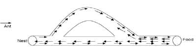
Fig. 1. Deposition of pheromone by the movement of ants

• III.    Related Work

The continuous research on congestion minimization for Mobile Ad-Hoc Network (MANET) using Ant colony Optimization (ACO) needs more and more new techniques. This section will elaborate the research related to congestion control. The traveling salesman problem (TSP) [1] is based on improved ant colony algorithm. In ACO algorithm, the main contribution is a study of the avoidance of stagnation behavior and premature convergence by using distribution strategy of initial ants and dynamic heuristic parameter updating based on entropy. The interesting algorithm is Ant Net algorithm [2], which is proposed for mobile ad-hoc network. In the improved version, more than one optimal outgoing interfaces are identified as compared to only one path, which are supposed to provide higher throughput and will be able to explore new and better paths even if the network topologies gets changed very frequently. This will distribute the traffic of overloaded link to other preferred links. Hence the throughput of the network will be improved and the problem of stagnation will be rectified in mobile ad-hoc network. Another interesting novel is Ant Colony Optimization [13], which is continuing to be a best paradigm for designing effective combinatorial optimization solution algorithms. In ACO application, ACO is one of the most successful paradigms in the Meta heuristic area. A newly interesting novel is Distributing Process [14], where the ant system paradigm is based on the population of agents. Each agent is guided by an autocatalytic process directed by a greedy force. When an Agent is alone then the autocatalytic process and greedy force is made that the agent coverage to a suboptimal tour with the exponential speed. Another novel is the Ant Colony Optimization (ACO), which is the meta-heuristic [13]  [15].The application of ACO algorithm is the traveling salesman problem and it is routing in the packet-switched networks. There are three main directions:

• •    The study of the formal properties of a simplified version of ant system.

• •    The development of Ant Net is for Quality of Service applications.

• •    The development of combinational optimization problems.

• IV.    Proposed Work

In this section we will discuss Swarm intelligence, Travelling Salesman Problem with MTSP, MTSP with ability constrain, Total Path distance and Path for creating a single path TSP using MTSP, ACO for MTSP, calculate the transmission Queue length, Total Queue Length, and Hop distance.

• V.    Swarm Behavior

The ant is inspired by the foraging behavior of biological ant colony, when they find paths to food sources. Each ant deposits a chemical called pheromone when they move from source to the destination and the foragers follow such pheromone trails. More ants are attracted by these pheromone trails .This natural phenomenon plays a role in developing and manipulating local information.

• VI.    Travelling Salesman Problem With Mtsp

Travelling Salesman Problem (TSP) is the most famous and is well-studied problem in the combinatorial optimization area. The multiple travelling problems (MTSP) are an extension of TSP. This problem relates with the accommodating real world problems where there is needed to account for more than one salesman. The MTSP can be generalized to a wide variety of routing and scheduling problems, for example, the School Bus Routing Problem and the Pickup and Delivery Problem. Therefore, finding a good optimal solution method for the MTSP is important and induces to improve the solution of any other complex routing problems. However, MTSP is a NP-complete problem for which optimal solutions can only be found for small size problems. It is known that classical optimization procedures are not adequate for this problem. Good heuristic techniques are necessary for solving MTSP due to its high computational complexity. Modern heuristic techniques, namely genetic algorithms and ant colony optimization, can be good candidates for this problem.

• VII.    The Mtsp With Ability Constraint

The MTSP can be stated as follows: There are m salesmen who must visit a set of n cities, and each salesman is defined to start and end at the same depot. In this problem, each city must be visited exactly once by only one salesman and its objective is to find the minimum of total distances travelled by all the salesmen. An example is depicted in Fig.1,where m=3,n=7.Several authors[6,7] suggested transforming the MTSP with m salesmen and n cities are into a TSP with n+m-1 cities by the introduction of m-1 artificial depots(n+1,...,n+m-1).The transformation of the previous example is depicted in the picture. Several authors have some researches on MTSP. Samerkae, Somhom et.al. have used Competitionbased neural network to solve MTSP with min max objective, and Linxin Tang et.al. have used the modified genetic algorithm to solve hot rolling scheduling problem, which is an example of MTSP. Proceedings of However, the resulting TSP is highly degenerate, when an MTSP is transformed to a single TSP since the resulting problem is more arduous to solve than an ordinary TSP with the same number of cities. While the general objective of the MTSP is to minimize the total distance which can be called minimum criterion, generally, there are m-1 cities always to select the nearest cities as their round trip. As a result, TSP which is made up of the left n-m+1cities is left. During the m salesmen, there are m-1 salesmen travelling only one city, and one salesman needs to travel the left n+m-1 cities. This is not up to the mustard. In practice, every salesman has the similar ability and the limit in ability. So the MTSP with ability constraint is more appropriate in the real world problems. We suppose the number of cities which are travelled by every salesman is limited.

• VIII.    Transformation From Mtsp To Tsp

The MTSP can be stated as follows: There are m salesmen who must visit a set of n cities, and each salesman is defined to start and end at the same place. In this problem, each city must be visited exactly once by only one salesman and its objective is to find the minimum of total distances travelled by all the salesmen. An example is depicted in picture, where m=3, n=7. Several authors suggested transforming the MTSP with m salesmen and n cities into a TSP with n+m-1 cities by the introduction of m-1 artificial depots (n+1,...,n+m-1). The resulting TSP is highly degenerate, when an MTSP is transformed to a single TSP since the resulting problem is more arduous to solve than an ordinary TSP with the same number of cities. While the general objective of the MTSP is to minimize the total distance which can be called minimum criterion, generally, there are m-1 cities always to select the nearest cities as their round trip. As a result, TSP, which is made up of the left n-m+1 cities are left. During the m salesmen, there are m-1 salesmen travelling only one city, and one salesman needs to travel the left n+m-1 cities. This is not up to the mustard. In practice, every salesman has the similar ability and the limit in ability. So the MTSP with ability constraint is more appropriate in the real world problems. Suppose the number of cities which are travelled by every salesman is limited.

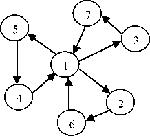
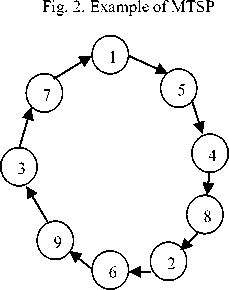
Fig.3. Example of Transformation from MTSP to TSP

In MTSP, where The MTSP can be stated as follow that there are m salesmen who must visit a set of n cities, and each salesman is defined to start and end at the same depot where m=3,n=7. Several authors suggested transforming the MTSP with m salesmen and n cities into a TSP with n+m-1 cities by the introduction of m-1 artificial depots (n+1,...,n+m-1). The resulting is n+m-1 = 7+3-1=9. So, there are city 8 and city 9, which are added in the giving example. In TSP city 8 is added between city 4 and city 2 and city 9 is added between city 6 and city 3.

In the fig4, each city must be visited exactly once by only one salesman and its objective is to find the minimum of total distances travelled by all the salesmen. Where m=4, n=12. So the MTSP with ability constraint is more appropriate in the real world problems. The numbers of cities are travelled by every salesman. It is limited. So, number of intermediate cities are three i.e. 13, 14, 15 (using n+m-1 formula).

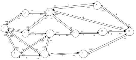
Fig. 4. Mobile Nodes with Distance and outgoing transmission queue

The Paths are, by which each salesman completed his tour and path distances are.

For Phase 1: P1:1-2-7-3-1 =25; P2:1-2-7-3-5-4-1 =36

We define the following variables and parameters Of MTSP:

First calculate total path distance.

Formula for calculate:

Table 1. Path (P) and Path distance(Pd) and Total Path distance(tdi)

Phas e Path and Path distance(Pd) Total   path   distance(tdi) (using equation-1) Phas e 1 P1:1-2-7-3-1=25(Pd);P2:1-2-7-3-5-4-1=36(Pd); others                  Pd are:38;35;36;38;36;54;58;48 etc. td1=(10465+1)*25=26,050; td2 =(1046-7+1)*36=37,440 Others are:39,482;36,400;37400;37, 440; 39,482;55,998;55,944;60,088 etc. Phas e 2 P1:1-3-7-2-1=25(Pd);  P2:1- 3-5-8-7-2-1=35 (Pd); Others                 Pd are:47;46;55;54;49;48;55;63 etc. td1=(1046-5+1)*25=26,050; td2=(1046-6+1)*35=36,435 others are: 48,786;47,702;57,053;55,944 ;5 0,862;49,920;56,980,62,205 etc. Phas e 3 P1:1-4-6-1=20(Pd);P2:1-4-6-5-3-1=25 (Pd);Others Pdare:38;39;23;36;24;50;49; 36 etc td1=(1046-4+1)*20=20,860; td2=(1046-6+1)*29=30,189 Others are:39,482;40,521;23,966;37 ,440; 25,008;51,850;50,764;37,440 etc. Phas e 4 P1:1-6-4-1=20(Pd);  P2:1-6- 4-5-3-1=29(Pd);Others Pd are:23;24;36;36;48;47;52;60 etc. td1= (1046-4+1)*20=20,860 ; td2=(1046-6+1)*29=30,189 Others are:23,966;25,008;37440;37, 440; 48,824;48,739;53,976;62,160 etc. tdi = (ni - l. + 1)*td           (1)

Where l_i is maximal number of cities salesman i ( 1 <  i <  M ) can travel, and n i is the real number of cities where the salesman i ( 1 <  i <  M ) ) has travelled, td_; is the total distance salesman i ( 1 <  i <  M ) has travelled, define the penalty function is n >  l .

Table 2. Total Path distance(tdi) and Path (P)

Phase	minimumTotal Path     distance (mtd i )	Path(P)
Phase 1	td 1 =26,050	1-2-7-3-1(P1)
Phase 2	td 11 =23,966   and td 12 =23,966	1-3-5-4-1(P 11 )  or 1-3-5-6-1(P 12 )
Phase3	td 1 =20,860	1-4-6-1(P1)
Phase4	td 1 =20,860	1-6-4-1(P1)

Then we calculate the minimum total distance (mtd ) for each phase, which is:

m mid = min ^td i=1

Using Equation No (2) we get minimum total path distance and path:

For Phase1: tdi= td1 =26,050 and Path ----- 1-2-7-3-1

So, single path is for TSP

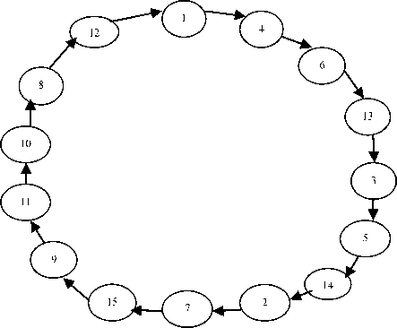
Fig.5. TSP with Single path

Here n is number of cities=12 and m is number of salesmen=4 .So, need number of intermediate cities are = (12+4-1) =3 are needed. These are 13, 14, and 15.

• IX.    Ant Colony Optimization For Mtsp

In Ant Colony Optimization (ACO), according to the characteristic of the MTSP, One salesman should first travel an amount of cities. In this way; all salesmen travel the total cities. The number of salesman is generated randomly in a certain range. Define the number of cities salesman i travels which is tni, ( (2 < tn; < l. ) where i=1… m).

^ tn = n - 1             (3)

The range of summation is 1 to m (range salesman is 1 to m). Where m is number of salesman, n is the number of cities, l i is the maximum number of cities salesman i can travel. Range of salesman is 1 to 4.

Using equation no 3 we find:

For phase1: ∑ tn₁ =5-1=4, ∑ tn₂ =6, ∑ tn₃ =7, ∑ tn₄ =6 , ∑ tn 5 =6 etc.

Table 3. Number of cities salesmen i travelled.

Phase	∑ tni =n-1
Phase 1	4,6,7,6 ,6 etc
Phase 2	4, 5,8, 9, 9 etc
Phase 3	3, 5, 7, 7, 4 etc
Phase 4	3, 5, 4, 4, 6 etc

• X.    Router Selection

Each ant spreads his/her trails, which are known pheromone. When the source node s wants to route the destination d which is known as natural topology using the initial artificial pheromone, each ant will be chosen its next hop or next node by probability P^k_i, j (t). First we calculate the distance between neighbor node and ith node. Then we also calculate the pheromone deposition and pheromone evaporation and residential pheromone on the link.

The Probabilistic path-selection is:

^AT kj^(t) = Д = mnAj )* ,'       ⁽⁴⁾

^{,           L}k                ^{,       d}i,j

Where Δτ^k_i, j (t) is the reciprocal distance L_k and L_k is the distance ant k has travelled the distance( d i,j ) and

Q=constant =minimum distance between ith node and its neighbor node.

So, we calculate the reciprocal distance

Δτ^k 1,2 (t)=6*1/8=0.75,Δτ^k 1,4 (t)=6*1/7=0.85

Δτ^k 1,3 (t)=6*1/6=1,Δτ^k 1,6 (t)=6*1/9=0.66

• XI.    Pheromone Deposition

Where τki,j(t) is the initial pheromone at kth node which is laying between ith node and jth node in the network at ‘t’ time and τki,j(t)=0.1 and λ is the rate of pheromone evaporate means ant “forgets ” previous decision for value λ=1,the pheromone evaporates randomly and find which is rapidly, when λ=0 results in slower evaporation rates, λϵ[0,1] and we assume that λ=0.6.

Then we calculate the pheromone deposition:

Δτ^{d k+1} 1,2 (t)=0.1+0.75*0.6=.55;

Δτ^{d k+1} 1,3 (t)=0.1+1*0.6=0.7;

Δτ^{d k+1} 1,4 (t)=0.1+0.85*0.6=0.61;

Δτ^{d k+1} 1,6 (t)=0.1+0.66*0.6=0.49

• XII.    Pheromone Evaporation

AT^ek+1 i,j (t) - T d ^k+1 i,j (t) * (1- X)             (6)

Where τ ^{d k+1} i,j (t) is pheromone deposition at k^th node, which is laying between node i and node j at t time and τ^{e k+1} i,j (t) is pheromone evaporation at k ^th node which is laying between node i and node j at t time and λ=0.6 .

Then we calculate the pheromone evaporation:

Δτ ^{e k+1} 1,2 (t)=.55*(1-.6)=.22,Δτ ^{e k+1} 1,3 (t)=.7*(1-.6)=.28, Δτ ^{e k+1} 1,4 (t) = .61*(1-.6)=.24,Δτ ^{e k+1} 1,6 (t)=.49*(1-.6)=.19

• XIII. Residential Pheromone

Δτ ^{r k+1} i,j (t) = τ^{d k+1} i,j (t) - τ ^{e k+1} i,j (t)           (7)

Where τ ^{r k+1} i,j (t) is the residential pheromone at k^th node, which is laying between node i and node j at t time and Δτ^{d k+1} i,j (t) is pheromone deposition at k^th node which is laying between node i and node j at t time and Δτ^{e k+1} i,j (t) is pheromone evaporation at k^th node, which is laying between node i and node j at t time.

Then we calculate the residential pheromone:

+(.37 ³ *.14 ¹ )+(.30 ³ *.11 ¹ ) =0.175

P^k 1,3 (t) = (.42 ³ *.16 ¹ )/(.33 ³ *.125 ¹ )

+(.42 ³ *.16 ¹ )+(.37 ³ *.14 ¹ )+(.30 ³ *.11 ¹ )=0.44

P^k 1,4 (t) = (.37 ³ *.14 ¹ )/(.33 ³ *.125 ¹ )

+(.42 ³ *.16 ¹ )+(.37 ³ *.14 ¹ )+(.30 ³ *.11 ¹ )=0.28

P^k 1,6 (t) = (.30 ³ *.11 ¹ )/(.33 ³ *.125 ¹ )

+(.42 ³ *.16 ¹ )+(.37 ³ *.14 ¹ )+(.30 ³ *.11 ¹ )=0.11

using equation no(8) we find that:

Δτ ^{r k+1} 1,2 (t) =.55-.22=.33,Δτ ^{r k+1} 1,3 (t) =.7-.28=.42, Δτ ^{r k+1} 1,4 (t) =.61-.24=.37, Δτ ^{r k+1} 1,6 (t) =.49-.19=.30

Then pheromone information is available and then every ant selects the next hop or next city independently. Suppose the ant k moves from city i to city j, uses the probabilistic formula, which is known the Baye’s probability theorem:

k          [τij(t)]α*[ηij]β ij        ∑[τil(t)]α *[ηil]β l∈Jik

Where α= related importance of the trail or pheromone trail=3.0;

β=relative importance of the visibility or sense=1.0;

Where α>0;β>0 and Where ɳi,j is the neighborhood node and ɳi,j =1/di,j .

using equation no(8) we find that:

P^k 1,2 (t) = (.33 ³ *.125 ¹ )/(.33 ³ *.125 ¹ )+(.42 ³ *.16 ¹ )

Table 5. Probability Theorem

j i	1	2	3	4	5	6	7	8	9	10	1 1	12
1		.1 75	.4 4	.2 8		.1 1
2	.0 9						.9 4
3	.5 1				.3 6		.1 1
4	.1 0				.2 6	.6 6
5			.1 0	.1 0		.6 0		.1 7
6	.1 4			.2 0	.5 5							.1 0
7		.4 4	.0 68					.0 42	.2 1		.2 2
8					.8 0		.0 73			.1 17
9							.3 1				.6 8
1 0								.0 50			.9 4
1 1							.0 14		.2 6	.7 0		.0 21
1 2						.8 2					.2 1

Table 4. Residntial pheromone

j i	1	2	3	4	5	6	7	8	9	1 0	1 1	1 2
1		.3 3	.4 2	.3 7		.3 0
2	.2 4						.4 2
3	.5				.4 2		.3 2
4	.2 7				.3 5	.4 2
5			.2 8	.2 8		.4 2		.3 3
6	.1 8			.3 3	.4 2							.2 8
7		.4 2	.2 7					.2 4	.3 5		.2 1
8					.4 2		.2 4			.2 7
9							.3 5				.4 2
1 0							.2 1				.4 2
1 1							.1 7		.3 3	.4 2		.1 8
1 2						.4 2					.2 9

• XIV.    Processing For Traffic Congestion Problem

Input:

d_i, j =Distance between i^th node and j^th node;

α= related importance of the trail or pheromone trail

β=relative importance of the visibility or sense; λ is the rate of pheromone evaporate

Output:

P^k_i, j (t)= probability matrix, τ ^{r    k+1} _i, j (t)=residual

Pheromone;

Begin:

• 1.    update values of path selection of Δτ^k_i, j (t)

• 2.    if(α>β)

• 3.    max of P^k_i, j (t);

• 4.    update value of τ ^{r k+1} _i, j (t)(residual Pheromone);

• 5.    else

• 6.    P^k i,j (t)=0;

• 7.    End if

End

• XV.    Calculate The Transmission Queue Length

  T i,j =1

  
  

  _-

  
  

^qi,j ∑ q i,j j ∈ N ⁱbi

Where q_i, j is the outgoing queue length(no of packets are sent ) is waiting to be sent to the link between i and j and N is all the nodes in the network and is N b ^[i] is the neighboring nodes of the node i. We have considered some random values as transmission queue length and T i,,j = transmission queue length. Using equation no (9) We calculate that T 1,2 =.8, T 1,3 =.7, T 1,4 =.7, T 1,6 =.8.

Table 6. Transmission Queue Length

j i	1	2	3	4	5	6	7	8	9	1 0	11	1 2
1		.8	.7	.7		.8
2	.2 5						.7 5
3	.7 2				.5 8		.7 2
4	.5				.7 5	.75
5			.7 5	.7 5		.75		.7 5
6	.7 0			.7 0	.9 2							.7 0
7		.8 3	.7 7					.8 3	.8 3		.77
8					.5		.6			.9
9							.4 3				.58
1 0								.6			.4
1 1							.7 5		.8 4	.6 7		.7 5
1 2						.37 5					.62 5

Now, arranging the path in ascending order with respect To Path calculate the Hop -distance or Number of Hop and Total queue length as follows in the table with their position:

Table 7. Hop-distance or no of Hop-count(Hd) and Total Queue Length(TQi,j)(For Phase-1)

Path(Phase 1)	Hop-distance or no of Hop-count(Hd)	Total Queue Length (TQ i,j )
P1: 1-2-7-3-1	4	3.04
P2: 1-2-7-3-5-4-1	6	4.15
P3:  1-2-7-3-5-6 4-1	7	4.85
P4: 1-2-7-8-5-3-1	6	4.35
P5: 1-2-7-8-5-4-1	6	4.13

Here for Phase 1: P1 is selected as Hop-distance of P1 is minimum and Queue Length of P1 is also minimum.

Table 8. Hop-distance or no of Hop-count(Hd) and Total Queue Length(TQi,j)(For Phase-2)

Path(Phase 2)	Hop-distance or no of Hop-count(Hd)	Total Queue Length (TQ i,j )
P1: 1-3-7-2-1	4	2.5
P2: 1-3-5-8-10-117-2-1	6	3.71
P3:1-3-5-8-10-11-7-2-1	8	5.16
P4: 1-3-5-8-10-119-7-2-1	9	5.68
P5: 1-3-5-4-1	4	2.53

For Phase 2: P1 is selected as Hop-distance of P1 is minimum and Queue Length of P1 is also minimum.

Table 9. Hop-distance or no of Hop-count(Hd) and Total Queue Length(TQi,j)(For Phase-3)

Path(Phase 3)	Hopdistance or no of Hop-count(Hd)	Total  Queue Length( TQ i,j )
P1: 1-4-6-1	3	2.15
P2: 1-4-6-5-3-1	5	3.84
P3:  1-4-6-5-3 7-2-1	6	4.92
P4:  1-4-6-5-8 7-2-1	7	4.80
P5: 1-4-5-3-1	4	2.92

For Phase 3: P1 is selected as Hop-distance of P1 is minimum and Queue Length of P1 is also minimum.

Table 10. Hop-distance or no of Hop-count(Hd) and Total Queue Length(TQi,j)(For Phase-4)

Path(Phase 4)	Hop-distance or no of Hop-count(Hd)	Total   Queue Length (TQ i,j )
P1: 1-6-4-1	3	2
P2: 1-6-4-5-3-1	5	3.72
P3:1-6-5-3-1	4	3.19
P4: 1-6-5-4-1	4	2.97
P5: 1-6-5-3-7-2-1	6	4.27

Here for Phase 4: P1 is selected as Hop-distance of P1 is minimum and Queue Length of P1 is also minimum.

• XVI.    Algorithm For Ant Colony Optimization

Each network node launches forward ants to all destinations in regular time intervals.

• 1.    The ant finds a path to the destination randomly based on the current routing tables and residual pheromone table.

• 2.    The forward ant creates Path using pheromone, for every node as that node ant is reached.

• 3.    When the destination is reached, the backward ant wants to start for creating a reverse path.

• 4.    The backward ant follows that path in reverse.

• 5.    Each of visited nodes is updated based on the routing table.

• 6.    The message ant is generated as link failure occurs and calculates the best link for new route setup.

Input:

q_i, j =the outgoing queue length

Output:

TQ_i, j =Total queue length

τ ^{r k+1} _i, j (t)=residual Pheromone

Begin:

if (Forward ant) {

Get the next node based on the value of qi,j if (the link is available) then

{

Update forward ant using network status and Send forward ant to the next node

} else if (no such link exist) {

Create backward ant and load contents (L) of forward ant to backward ant and Send

Backward ant towards source along the same path P as forward ant

}

} if (backward ant)

{ if current node is source node

{

Store path distance (Pd);

Then kill the backward ant;

Update routing table and residual pheromone (τ ^{r k+1} i,j (t)) } else

{

Proceeded the backward ant on to link available on queue

Update routing table and residual pheromone (τ ^{r k+1} _i, j (t)) } if (next node is not available)

Kill backward ant

Else { if( link failure) then Update forward ant with network status as failure and stop sending information (data) or outgoing queue (q_i, j ) Send message ant to the previous node regarding link failure update table for alternative path (P) and path distance (Pd) based on link stability parameter for path is recovered or restore.

}

} // End of proposed algorithm

End if

End

Now we compare the Hop-distance and Queue Length among four phases.

Table 11. According Hop-distance or Number of Hop, Load and Total queue Length and position of the paths.

Position	Hop-Distance or No of Hop count (Hd)	Load(L)	Total    Queue Length(TQ i,j )
1	P41	P41	P41
2	P31	P21	P21
3	P21	P31	P31
4	P11	P11	P11

From above it is cleared that the sum of position path is P41 (P1, for phase 4).This is minimum. Hence path P41 (P1, for phase 4) is selected.

• XVII.    Processing For Load Contains Of PathSelection

Input:

q i,j =the outgoing queue length;

T i,,j = transmission queue length

TQ_i, j =Total queue length

Hd= Hop-distance of path-selection

Output:

L=Load contains between path-selection.

Begin:

• 1.    if(TQ_i, j & Hd are small between the Paths)

• 2.{

• 3.    Load(L) is available;

• 4.}

• 5.    else

• 6.{

• 7.    Load(L) is not available;

• 8.}

• 9.    End if

• 10.    End

Table 12. Compare Hop-Distance or number of hop and total Queue Length among Four Phases

Path	Hop-Distance or No of Hop count (Hd)	Total Queue Length(TQ i,j )
P1(for phase 1,(P11))	4	3.08
P1(for phase 2,(P21))	4	2.5
P1(for phase 3,(P31))	3	2.15
P1(for phase 4,(P41))	3	2

• XVIII.    Conclusion

The mobile multi-hop ad hoc networks are flexible networks which do not require preinstalled infrastructure. The main challenge in MANET is still the routing problem due to the mobility of nodes. Various approaches were introduced, but no one fitted best for all applications. In this paper we present The Ant Colony Optimization for MTSP and Swarm Inspired Multiple Data Transmission with Congestion Control in MANET using Total Queue Length. We explore the property of the pheromone deposition by the real ant. The proposed algorithm using path pheromone scents constantly updates the goodness of choosing a particular path by measuring the congestion using hop-distance and queue length into the network. By incorporating the wireless medium information from the MAC layer into the routing decision procedure our algorithm can prevent forward data traffic across congested areas. Our future work includes the implementation to improve the algorithm and also we are using ns-2 simulator for our further investigation which include experiments with high network load.

Acknowledgment

We thank anonymous referees for their suggestion to revise the paper. Dhriti Sundar Maity is grateful to Global Group of Institution (GGI), Haldia, Purba Medinipur, West Bengal, India, for the environmental support to do this.