Neural network forecasting algorithm as a tool for assessing human capital trends of the socio-economic system

Автор: Ketova Karolina V., Vavilova Diana D.

Журнал: Economic and Social Changes: Facts, Trends, Forecast @volnc-esc-en

Рубрика: Modeling and forecast of socio-economic processes

Статья в выпуске: 6 т.13, 2020 года.

Бесплатный доступ

The article addresses the issue of neural network forecasting of human capital size, structure, and dynamics. The object of the research is the socio-economic system. The subject of the study is the practice of applying neural network models to forecasting socio-economic indicators, human capital in particular. The purpose of this work is to apply neural network modeling and adapt its algorithms to build a forecast of the studied indicator for the future. The statistical base is data on demography, the investment volume in human capital of the regional economic system, as well as the indicators of socio-economic development. The investment volume in human capital is determined by budget and private citizens’ expenditures. To forecast the human capital dynamics the authors used the values of investment volumes the forecast of which, in turn, is built using a neural network modeling. The neural network model used in this study is a multi-layer fully connected perceptron with a sigmoid logistic activation function. Neural network modeling of forecast values of investment volumes has shown its effectiveness. Human capital assessment for the period of 2000-2018 and its forecast for the period of 2019-2023 are based on the example of the regional economic system of the Udmurt Republic. Our calculations show that the highest growth rate of the studied indicator has been demonstrated since 2013, and its further increase is predicted. The results obtained correlate qualitatively with the dynamics of changes in the Russian human development index, determined by the UN experts. The proposed method of calculating and forecasting human capital can be used to assess and compare the socio-economic situation of Russia’s regions.

Еще

Human capital, neural network modeling, algorithm forecast, investments, socio-economic system

Короткий адрес: https://sciup.org/147225499

IDR: 147225499 | DOI: 10.15838/esc.2020.6.72.7

Текст научной статьи Neural network forecasting algorithm as a tool for assessing human capital trends of the socio-economic system

Building development strategy for the socioeconomic system which is based on a stable growth of its indicators is an urgent task. When solving this problem, a mathematical modeling tool should be used, as it allows building economic dependencies for the future with a given accuracy.

The strategy for the socio-economic system development involves the construction of schemes for financing industrial and social spheres of activity. The production sphere is characterized by the structure and size of production capital (PC), the methodology for calculating which is well known. In recent years, human capital (HС) has been increasingly used to assess the social sphere which is a leading factor in determining high development rates in modern economy. Consequently, issues related to the human capital study become important and relevant.

The HC concept appeared in science in the 20th century in the works of American scientists-economists J. Mincer [1], T. Schultz [2] and G. Becker [3]. The impetus for the HC theory creation was statistical data on the growth of the developed countries’ economies. The analysis of real processes of development and growth in modern conditions has led to the HC study as the main productive and social development factor. For creating the foundations of the human capital theory, the Nobel prizes in Economics were awarded (T. Schultz in 1979 and G. Becker in 1992). S. Kuznets made a significant contribution to the HC theory creation. He showed that human capital is the main dominant factor in the possible stable growth of developing countries’ economies [4].

Among the scientists who have made the greatest contribution to the HC theory development are M. Blaug, M. Grossman, M. Perlman, L. Thurow, F. Welch, B. Chizwick, J. Kendrick, R. Solow, R. Lucas, C. Grilliches, I. Fischer, E. Denison and other economists, sociologists and historians. Among modern Russian researchers dealing with the HC problems, we can mention S.A. Dyatlov, R.I. Kapelyushnikov, M.M. Kritskii, S.A. Kurganskii, O.I. Ivanov, and others. There are several approaches to assessing human capital. The models of I. Ben-Porat [5], D. Heckman [6], A.S. Akopyan, V.V. Bushuev and V.S. Golubev [7], S.Yu. Malkov, K.A. Bolotova, and O.I. Davydova [8].

Building a general methodology for the HC calculating is a rather difficult task, as there is a large proportion of subjective assessments when modeling it. There are also different positions on the basis of which the HC concept is formulated, in particular, it can be studied from the point of view of the quality of human life

[9], its ability to perform high-performance activities [10], as the amount of income that a person can receive [11] or as the amount of investment in the social sphere [12]. In 1990, the United Nations Development Program proposed a methodology for assessing the HC level based on the calculation of the human development index ¹ .

Whatever approach the researchers would chose to assess HC, it is important that at present this indicator should be considered as one of the most important factors that ensure the socio-economic system development [13–17].

In our work, we used an integral economic and mathematical HC which includes its quantitative and qualitative characteristics [18]. Based on this pattern, the HC value is calculated. We performed the HC forecast using a neural network algorithm.

Neural network modeling is one of the mathematical methods for studying various processes and phenomena. It is used for solving problems of data mining and forecasting [19–22].

Initially, artificial neural networks (ANN) were constructed as a result of studying the nervous system of a living organism [23]. Neural network is in a certain way an analogous to the brain in terms of its qualitative structure and the number of neurons it contains.

In recent decades, neural networks have been widely used for forecasting. Forecasting is one of the most popular, but also the most complex tasks of ANN. The forecast error always depends on the selected pattern, the availability and quality of the source data.

Neural networks have the following advantages in making forecasts: effectiveness in solving unformalized or poorly formalized tasks; resistance to frequent changes in the environment; efficiency when working with a large amount of contradictory or incomplete information. These advantages are relevant including the cases when applying neural networks to the forecasting socio-economic processes and phenomena.

The advantages associated with the use of neural network patterns and their modifications in the analysis of socio-economic processes and phenomena are presented in [24, 25]. The authors show that neural network patterns have the property to take into account the influence of implicit factors and include non-obvious mathematical connections in the study that are difficult to find using classical econometric patterns, the regression ones in particular.

ANN were first mentioned in the 1940s. It is recognized that the neural networks theory was designated as a scientific direction in 1943 in the work of W. McCulloch and W. Pitts [26], where the authors showed that any arithmetic or logical function can be implemented using a simple neural network. Among the fundamental works, we should also highlight the pattern of D. Hebb [27] who proposed the first learning algorithm in 1949. In 1958, F. Rosenblatt constructed a pattern of a perceptron containing a single layer [28]. After some cooling to the ANN, a new wave of interest emerged in the 1970s. Thanks to the research of T. Kohonen, S. Grossberg and D. Anderson, the foundation was completed, on the basis of which it became possible to build and use multi-layer neural networks [29; 30]. In 1974, P. Werbos developed a basic algorithm for training multilayer neural networks which was widely used in practice [31]. Among the researchers in the ANN, one can also distinguish M. Minsky [32], K. Fukushima [33], J. Hopfield [34], S. Haykin [35], R. Hecht-Nielsen [36], and others. Recent research on the formation of

Figure 1. Research structure

Indicators of the main directions of Socio-economic development

Algorithm for neural network modeling and forecasting of human capital components

Results of solving the problem of forecasting the qualitative human capital components

Algorithm for modeling and forecasting the human capital value

Results of solving the forecasting problem qualitative human capital components

Forecast of the human capital size and dynamics

Source: own calculations.

neural network modeling algorithms, dynamic series analysis, and forecasting is presented, for example, in [37–40].

We consider the problem of forecasting the human capital of a socio-economic system based on a neural network algorithm. The study structure is shown in Figure 1 . Indicators of socio-economic development directions are determined in accordance with the work [41]. The neural network modeling algorithm and forecasting of the HC components allows making their forecast. The algorithm for modeling and predicting the HC value uses the results of forecasting the HC components to calculate its total value.

Economic and mathematical pattern of human capital

The HC carriers are demographic elements each of which is characterized by age τ at a time t. The number of demographic elements determines the quantitative HC characteristics. To implement an effective demographic policy, it is of great importance to conduct research such as the analysis of modern demographic processes and forecasting the population size and structure based on it, taking into account the specifics of birth rate, life expectancy, migration processes, and mortality.

Figure 2 shows the dynamics of the total population for the 1997–2018 period using the example of one of the regions of the Russian Federation – the Udmurt Republic (UR). Figure 3 shows the dynamics of fertility and mortality.

The calculation of the HC value should be carried out taking into account the demographic structure. The distribution of demographic elements by age ρ ( t , τ ) is important in this case. Under the demographic element here and further we will understand a representative of the population – an individual who at the time t under consideration is characterized by the age τ . Figure 4 shows the age distribution of the UR population for 2008 and 2018, respectively. The function ε ( t , τ ) sets the percentage of the age τ population participating in social production per t year. The problem of modeling and forecasting demographic dynamics is presented in detail in this work [42].

To calculate the human capital value of the economic system Н(t) , the pattern [18] is used according to which the total value of the

Figure 2. UR population dynamics

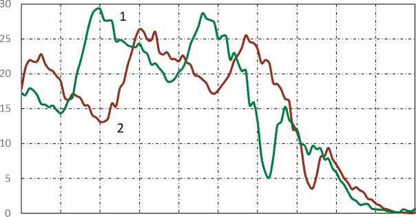
Figure 3. UR population dynamics of birth rate (1) and death rate (2)

Р ·10^-6, peop.

1,62

Р ·10^-3, peop. 26,0

1,60

24,0

1,58

22,0

1,56

20,0

1,54

18,0

1,52

16,0

1,50

t , year

1997 2000 2003 2006 2009 2012 2015 2018

14,0

t , year

1997 2000 2003 2006 2009 2012 2015 2018

Source: Total population of the Udmurt Republic. Available at:

Source: Population of the Udmurt Republic by gender and age. Available at:

Figure 4. The density of the UR population distribution by age: 2008 (1); 2018 (2)

ρ·10-3, peop.

0 10 20 30 40 50 60 70 80 90 100 τ, year

Source: Population movement of the Udmurt Republic. Available at:

population HC participating in social production is determined from the expression:

H ( t ) =j f a i h i ( t,T ) 6 ( t,T ) p ( t, T > . (1)

0 i = ¹

Functions hi(t,τ) are the quality HC components: health i=1, education i=2, and culture i=3. Investment in health raise the general level of health in society which contributes, on the one hand, extending the economically active life of individual demographic item, and, on the other hand, the increase in the number of economically active population elements due to the reduction of mortality. Investment in education contributes to improving the overall skills level in the regional labor market, opening up the greatest reserves for improving the modern economy efficiency. Investments in culture improve the

It is obvious that the coefficients of disposal

human environment, form moral values, and increase the creative potential of the individual which, of course, affects the region’s socio-

v_i are weakly time-dependent. The age dependence for functions v_i = v_i(τ) (i = 1, 2 ) is taken as follows:

economic development. [0, т<т ai ,

The specific (per demographic unit) HC ^v i ⁽ ^T ⁾ [( s X t , t ) + p i ( t ,т)){ехр[еХт - т ai )]-1}

T < T < T , ai m m ,

average value is determined by a linear combination:

Where the unknown parameters ( s_i , ε_i ) are determined from the conditions:

h(t, r) = a 1 h 1 (t, r) + a ₂ h 2 (t, r) + a ₃ h₃(t, r ), (2)

а е( 0,1 ) ; I a = 1 , (3)

. i =1

where: α _i are the corresponding weight coefficients for the HC components; values h _i ( t,τ ) are measured in monetary units.

During the research, the hypothesis of the equivalence of the HC components was accepted: « = 1/3, i = 1,3.

The evolution of each of the HC components is described by the equation:

( 5 i (t, T) + p i ( t , т)){ехр ^[e i ( t m —-г a ,.^)] — 1 ^}= 1 , (9)

д h _i(t, t) д h _i (t, t) dt ⁺ дт

—V h i⁽ t, т) + S i ⁽ t, т) + P i ⁽ t, т) .(4)

In formula (4), the following notations are used for each HC component: s_i = s_i ( t,τ ) – specific state expenditures; p_i = p_i ( t, τ ) – specific private investment; v_i = v_i ( t, τ ) – the coefficient of disposal which is estimated using the identification algorithm [43].

The initial conditions for t = t ₀ are as follows:

ht(t₀, r) = h toGO, ( i = 1,2,3 ), (5)

where: h_i ₀( t ) – known functions.

At the left end of the demographic curve, the boundary conditions are as follows:

h_t (t,0) = 0, ( i = 1,2,3 ); (6)

at the right end, where i = 1, 2 the following should be written:

h i ⁽ t, да ) « h i (t, r _m ) = 0 , (7)

where: τ_m = τ_m(t) – survival time δ of the population’s percent ( δ = 1–5% ) .

^T m

J[ 5 , .( ^ , т) + р ( , т)] d t =

= J^{( s i ⁽ t , ^т) + P i ⁽ t , ^T)⁾⁽exp^[e i ^(т — ^т ai ^)] — 1)} h ⁽ t ,^т) d ^т .

^т ai

^т m

Here τ_ai is the upper limit of the active period of physical condition ( i =1) or work activity ( i =2).

When performing specific calculations for the UR economic system, we have analyzed demographic data for the period of 2000–2018, and found that the age limit of the economically active age of the UR population is 20–60 years old.

Unlike other components, the cultural HC component is not subject to disposal, so v ₃ ≡ 0.

For the equation (4) that sets the evolution

of the HC components, the age distribution of the specific components of state budget expen-

ditures s_i (t, τ ) is determined by the formulas:

5, (t ,T )=^ r SN^t) , i T 2 Ni

^N‘ J p ( t , t ^d ir

^T l Ni

Sn. ( t ) =

^SNi ⁽ ^t, ^T ) , ^T ^e[^ 1 Ni^, ^T 2 Ni ^] , .⁰, ^T ^^[^ 1 Ni / t 2 n ] -

Here S_Ni (t) is the amounts budgeted for the corresponding item of expenditure N_i ( N_i – numbering of budget items spent on health ( i =1) , education ( i =2) , and the development of the cultural HC component ( i =3)) . In accordance with formula (11), these amounts will be distributed evenly over the corresponding periods of a person’s life [ τ _1Ni , τ _2Ni ] and the number of demographic units in these periods.

For equation (4), the age distribution of the specific components of private expenditures p_i ( t, τ ) aimed at HC increasing is written by analogy with (11), assuming that a person uses various amounts of money spent on health ( i =1) , education ( i =2) , and culture in different periods of life ( i =3) :

Pl ( t )

Pi⁽ ^t ^,T ) = £ 7;---------- ,

‘ J p ( t , t ) Т

^T 1 i

_t ) = ( P ⁽ t^, ^T ), ^т ^е ^Т 1 = ^, ^т 2 ; ] , ⁷ I^0, ^T £^[C^, ^T 2 i ^] .

Algorithm for neural network forecasting of human capital

Let us build a neural network for solving the problem of predicting human capital. Figure 5 shows a neural network element – a neuron with m inputs and an output. This construction of a neuron is called a perceptron. An artificial neural network is a way to assemble neurons into a network to solve certain tasks. The trained artificial neuron works as follows: each input is multiplied by certain weights; then everything is summed and run through a nonlinear activation function, and the result is fed to the output. All the neurons are collected into layers. Basic computing operations are performed on internal hidden layers.

Another task is to train the neuron. Training consists in finding the correct weight information which is adjusted based on the task and error (the difference between the calculated and ideal output values). For this purpose, the error back propagation algorithm is used.

The input data is summed with weights w : m ^j d = 2 w ^x . The neuron s output has a logistic activation function f(D) (Fig. 5) that converts the weighted sum D of the incoming signal ( Fig. 6 ).

To forecast the investment volume in the social sphere, we construct a complex k -layer neural network with m inputs and l outputs ( Fig. 7 ). The input data in the neural network pattern are the volumes of budget { S , } n = and private { P i } investment in the HC, the indicators of socio-economic development directions { I i } "‘ 8 . The deflator index K is used to account for inflationary processes. The output data of the neural network is the projected monthly volumes of budget and private investments in ~ n =3 ~ =3

HC: { 5 , }=, and^{ P i } =,.

For our task, we will consider budget investments in healthcare ( x ₁ ), education ( x ₂ ), and culture ( x ₃ ), as well as private investments in healthcare ( x ₄ ), education ( x ₅ ), and culture ( x ₆ ). The amount of investment in the social sphere

Figure 5. Artificial neuron Figure 6. Activation function

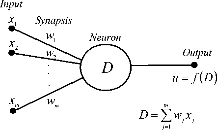
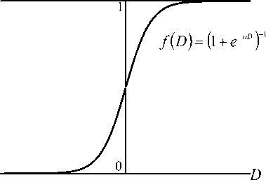
Figure 7. Neural network pattern used to forecast investments in human capital

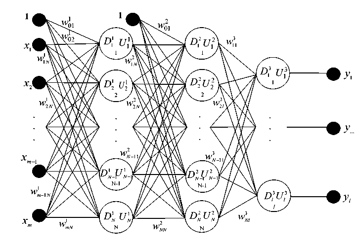
Source: own calculations.

depends on many factors and environmental conditions. In the work of S.A. Ayvazyan

[41] identified indicators that most strongly affect the quality of the social sphere, namely:

gross regional product ( x ₇ ), average per capita monetary income ( x ₈ ), production of goods and services per capita ( x ₉ ), the area of housing commissioned ( x ₁₀ ), the number of registered crimes ( x ₁₁ ), natural population growth ( x ₁₂ ), mortality in working age ( x ₁₃ ), the minimum required monthly income ( x ₁₄ ).

Thus, ^{ ^S, ^} " =’ = ^{ x ,, x 2, x 3 ^} , ^{ P i ^} "3 = ^{ x 4 , x 5 , x 6 ^} ,

^{ Il ^} j =1 ^{ x 7, x 8, x 9, x 10, x 11, x 12, x 13, x 14 ^} , ^K x 15^.

We will construct a neural network pre- diction algorithm for any case with any number of input variables. Figure 7 shows the neural network pattern underlying the algorithm.

Each layer of the neural network pattern contains N_p neurons p =1,…, k .

We will use the following notation: w ^ the weight coefficient of communication connecting the signal coming out of the ( p -1)

layer of the i -th neuron and entering the j -th neuron of the p -th layer. For each layer, the coefficients are represented as a matrix with the size ( N p - 1 + 1 )x N p :

W = ( w p ), p = 1,.., k ; i = 0,.., N j _ ,; у = 1,.., N _p. (13)

From an algorithmic point of view, the output values of the zero layer u ⁰ _j should be equated to the signals entering the neural network x , x ≡ 1 :

j ⁰

u 0 = X j , j = 0’"’ m . (14)

In other layers, the output values of neurons are calculated:

u 0 = 1, uj = f ( dj ) p = 1,.., k , j = 1,.., N j , (15) where f ( d j ) — nonlinear activation function of the, f ( t ) = ( 1 + e - "‘ )^-1 , a — a coefficient.

Let us denote d _j ^p as the input signal in j -th neuron of the p -th neuron layer which is determined by the weighted sum of the incoming signals:

Np -1

d j = Z w p u p -1 , j = 1,., N_P . (16)

i =0

The output values of the last k -th layer should match y_j :

y j = u k , j = 1,.., l , (17)

The training process consists of adjusting the weight coefficients w _i ^p _j . Based on the information about the values of variables at known points in time, the network determines their most likely values for the future. Statistical information on socio-economic indicators is divided into two sets: the training set and the test set which is a section of the retro-forecast.

To train the network, input data is fed to the inputs x _q = ( x_q ₁ , x_q ₂ ,…, x_qm ) and the output values of the network are compared with the ideal (actually set) values, r _q = ( r_q ₁ , r_q ₂ ,…, r_ql ), q =1,…, n .

The training set of data is used to implement an algorithm for training a multi-layer neural network using the method of back propagation of errors which is related to gradient optimization methods [44]. To determine the network weight coefficients W = ( w p ) , the network training error is calculated using the formula :

^Eq ⁽ ^W )= ¹ £ ⁽ У ф - Г ⁾² , 4 = Ъ", ^П , ⁽¹⁸⁾

2 j =1

where y_qj is j -th output when the input of the q -th image.

When submitting the q -th observation, the coefficients will change as follows:

In the component form, the expression (20) is represented as:

5E„ wp (q^ = wP (q - 1)+A wp , AwP =-X---- . (21) ij ij ij ij p

5 w p

Vector components (21) are written as follows:

d E d E d u p d d p

___q_ ____ q___j__ j d w p d u p d d j d w^p ’

∂ujp where partial derivative ∂dp in accordance with the derivative of the loj gistic function ft) = a f (t)(1 - f (t)) is represented as:

d d

duj j = a-up -(1 - up).

5 d p j ^{V j)}

Let us introduce a new variable δ ^p _j as follows:

, 5E_a d u f

8 ^f = —q- -j- ,

' 5u 8dp jj

^dEq = ^Nf ¹ ⁵ ^Eq 5 U ⁺¹ 5 ^df ⁺¹ = N p +1 5 E q Э Н^ w ₊, d u p и d uf ⁺¹ d d , ^-+1 d u p и d u , ^p ⁺¹ d d ^- ⁺¹ j ^{. (25)}

Then δ ^pj we can recursively calculate through the data of the (p +1)-th layer 5 p ⁺ ¹ :

⁵ P =

N p +i

Z 5 p ⁺ ¹ w p + i =1

• a • u - • (1 - u p ) .

When p = k from (16), (23) and (24), equating u p = y_qj , we find:

5/ = [u p - r_qj\ • a ■и¹-' • (1 - u p ) . (27)

W ( q ) = W ( q -1) + (-X-V E_q ) , (19)

where W ( q ) — the vector state W after training the network by the q -th observation; Xe ( 0;1 ] — training rate of the network; V E q — gradient of function E q WW ) , when the input is submitted q -th image :

V ^Eq

)

Sw P

< wj-j 7

j = 1,

N p . (20)

The last multiplier in formula (22), according to (16), is equal to: ^∂ ^djp = u ^p ^-1 .

∂wp i ij

As a result, based on the formulas (21), (22), (24) we get the difference scheme:

j. ( q ) = W ( q -1 ) -X5 j u p ^- ¹ . (28)

In order to train the network, you need to normalize the input and output data in the area of their definition. If it is known that x_j ∈ [ a_j – h_j ; b_j + h_j ], then the normalized input data has the following form :

x = x qj —⁽ ^b J ⁺ a/i/ ^ q 4b, - a, )/2 + hj

q = 1,

n .

Table 1. Budget and private investments aimed at the UR human capital development for 2000–2018 in the current prices

Е ей >-

ОТ тз с 3

го

СП тз

Х2 ГО

X о о го от го

73 С го

о ел

73 3

-Q 73

О ГО

о от с о о

СЕ ТЭ

О х:

о от о

т с о Q-X

см со со

cd со CD

О) со

а> со со со см

го

ГО

сэ

ГО

сэ

см о

см

со

OD го

сэ

OD об

го

СМ

со см

ОС

,с от

73 с ^ го о С5Э

73 3

Х2 го

о о го от

73 с го с о

го о 73 о

с го "от

от 3

СЕ о х:

*о

о С5Э

73 3

Х2

го а> 73 о

о х:

Е о

от о

т с о Q-X

го

3 Q-о О

СЕ ^

о х:

с о Е

от о > ,с

го >

со ОО

со со ОО

го со го

аэ со со со

со

см UO о

ГО

со со

ОО

LTD

со

го

а> со со со о

го

LO co

ГО

га

ГО

о о со см со

со

СО

ГО

го

см со сэ см

сэ

со

см со см ио

а> со

со со

со

СО об ОО го

оэ

см го оэ

го

cd co

г-

го

ОО

га

со

о го

OD го

сЗ

ГО со

го

со

го

со см

СО

об g

го го

о со ГО см

см о>

со

ГО ОО

ОО

о оэ го ио

ОО

со

СО

сэ

СО

ГО

со об

ГО со

со сэ о о со

ОО

со

го

га

со го

ГО

го

0D ГО

ГО

со

аэ оэ

о о>

го го

го

ОО

ио ио го

ио

со

ГО

СО

ГО

га

о со со

см

го

об го

га

об

оэ со

со см

га

со

ГО

со

со ГО

оэ оэ со

со

ОО

га

оэ со

ОО

СО

CD го

со

ГО

°? S со

со

LTD

га

ГО

го го со со

ОО

со

LTD

ГО

со

го

го со

го

о о см

го

ГО со

га

со

го о> со

об со CD

об

ГО

со g

га

со S ио

га

ГО

го

ГО

см го

см

со

OD СО

со со ГО

ОО

О)

со со

UO СМ о>

см

об

ГО СО

ОО

со см со

со

CD го

га

сэ

оо

ОО об

ОО

ио ио

сэ

га

со о о

со

ОО

го

О)

сэ

со см

со см ио со

об

ОО го

об

га

ио со ио го

го

со со

ГО

га

об

ОО

со сэ

со

ГО

об

ГО

°°

го со о ГО

ю со

OD g

со го CD

со оэ со

со оэ ГО

го

сэ

ГО

со ио го

об

со

га

со со

ОО

СО об

о со

ГО

со

СО

ГО

го см оэ со го

ГО

со ио со о

ей о>

Е го

е i—

t о Q-от

73 С го

х:

го о

х: ,с от с о Е от о >

,с

о ел

73 3

СП

^Е

^Е VI

го о 3

73 о

,с

с о

от о >

,с

о ел

73 3

СП

ОО

со

^Е

"з о

,с

с о Е

от о > ,с

о СП

73 3

^Е

го о н

^Е

го о н

^Е

го о н

о го о

"ей тс

"о

со

"о

"ей

"о

Е о

о го о х:

го о х:

с о

от о > ,с

о С5Э

73 3

го о

73 о

с о

от о > с

о С5Э

73 3

"з о

,с

с о

от о >

,с

о С5Э

73 3

о го о х:

го о х:

с о Е

от о > ,с

о го > oZ

го о

3 73

О С

с о

от о > с

го >

о 3 от о

73 С го о

3 "з о ,с

с о Е

от о > ,с

о го > oZ

со

ОТ ■О с

ш ОТ "О

15 о

■О с

ш ОТ 73

■О ф

те

о ОТ

о о

сс :э

те

х" ш

от

о см

со

со от от от

со

ОО

от

ОО

от от

со

со ю со

со см со

от от

ОТ от

ОТ

см

ОТ см со о от

сс

,с

V) 73 с 3

го

ф СП 73 =

-Q

го 5

ф ф го от 73 с го с о

го

ф 73

с го от от =

сс ф

*о

ф СП 73 = Х2

го

ф 73 ф

ф х:

Е о

от ф

73 с ф о. X

от" от

ОТ

от ОТ от см

о го = о. о о. сс

ф х:

с ф Е от ф > ,с ф го > oZ

от от

от

ОО

о со см о> со

1 1 аз с

С о

С 8"

2 о

■К

го Е = го 5

I 1

1 || i Ц те g § to гм =5

1 1 1 s f 1 о Е +5 => "□)

■о те £ CD Q-

.го §-5

ар Е £

° So и “

.те ,с

s II го го

о те Е

1 “ S

са ^ ^ 'о ~ о те со 12 .. = ь °

-те "сб о аз Ч те ” аз ел х со to те с гм g ° go з_{ш т}
^ СО " -Q си СП

ОТ

со от со

со см

ОО

ОТ

ОО

со

от со

от

LO со со со со

от

от от от

ОО

от от

со со от

от

от от

ОО

от см от со

ОО

от

ОО

от со от

со см от

от со

со

СО СО

от

ОТ

S от

от со см

ОО

от

от от

от

от со

со со со со

от

СО

от

°°

от

со от от

от

со

от

CD со

от

от от от

о о

см со

го

ОТ

от

ОО

ОТ со ОТ

о от

со со см

ОТ

от

СО со

ОТ

от со от

LO со от

сэ

от

от от

СО от

ОО

со см о от

от от

ОО от

от от

от

от со о> от

со

от

ОТ

см от

ОТ со см

от

ОО

от со

со ю

от

со от

от

ОО

о о со о

от

от от

от

от от от от

от

о о со

со со

со

см о со

см

от со

от

со от со

от

со

от от

от со со

см

от

о§

от от

°°

см от от от о от

от

ОО от

от

S от от см

о со

от

ОТ

ОО

от

от о со

см

от от

от

со о от от

от

со

от

со см

СО

ОТ

со о о со ОТ

от

ОО

от

ОТ

S от

со

от ю

со от

см

от

ОО

об

от от от

от

от см от см со

от

от от от от ОО

со о со со см

от

от со

от от

со

ОО

со

со со со со

со

ОТ

от

от со

от

ОО

от

от об

ОО

от со

от со о со

см

от от от от

от

со от о см

с о

ОТ

■О

те

ф ОТ 73

^Е

го о =

73 ф

с ф

ф > с

ф СП

73 =

СП

ОО

^Е

,с

с ф

ф > ,с

ф СП

73 =

^Е

го о н

^Е

го о н

^Е

го о н

"те

"о

со

"о

"те

S 2

"те ^ с с .о о

о о

о 11

"о

Е о

о о. от

73 С го ф

го о

х:

го ф х:

с ф Е

от ф > ,с

ф СП

73 =

го о

= 73

С ф

от ф > с

ф СП

73 =

"5 о

,с

с ф Е

от ф >

,с

ф СП

73 =

о о.

73 с го

го о

х:

го ф х:

с ф Е

ф > ,с

го > £

о го о = 73 Ф С

с ф Е

от ф > с

ф го > £

= от ф

73 с го

"5 о ,с

с ф

ф >

,с

ф го > £

ТTable 2. Dynamics of basic indicators of the main directions of the UR socio-economic development for 2000–2018

s	co	s	co	co	co	g	g	*	g
g		8	g	co		s	g	*	8
g	g	co	cd	8	CD	g	g	*	g
g	co	g	co	Si	8	g	8	*	g
	g	8	8	g	cm	g	g	*	8
g	g	co	s	co	CD	g	g	*	8
§	oo	g	g	co	CD	g	g	*	g
g	g	co	co	co	Si	co	g	*	g
g	s	8	4	CM	g	co	g	*	co
g	g	co	co	CM	g	g	g	*	g
О "co о	Ё 6	E \| E	ro CO CO О ^ о ® 2 ^	E Ё E	E	1 CO s	E s	1 E 2 5 E ^EE ^ 2 E

co		co	g			g	CM	*	8	E E CT CT LO .5 .9 8 ® ® CD CD о S S о сл <л E S s s CM Ё jo tc tc ° “ ” о ra rare CD Q) CD 00 "o 1^2 ex? ^ ^ ^ Ф ^ 'ey 3j 5 5 ^g<< -zC CO f-C co co ™ E О E E S «i E % т ® ® "ст В ш ^ "o "o 3 § 1 3 ^Q Q- ^ ^ "o +^ co co CO — m ^{c c} C ^w CD CD ^ ТО ТО о Д Д o co "A -= о о о _ ™CO q_oOCO д ф ^ о to о о ^ О CJ ” ™ ° ° s = ОС — = го g -пОо<ФФи Etro.^oo g ^гогоЁЁгага^ g \| ^Е s 5 се — ссз га го о Е § ® -Е_с§”-оЕЕ< 5 ^ - 2 5 D о о -= o_™g?c6°?raro^ га _-₅ССС=5С1-С1-^ га "=Ее,ЪЁЁ8 С/D О ‘ А О CD г— "^1—' "^1—' О Ё..^Ега\|’-гага««Р S "v> \п ТЗ ТЗ 33 о 2A.^Bo=SOCDCDCO О ^O(VDZCCCD_CCCC^ * сл^схГсо'^-'ю'сВ'г^'оо'
g	g	g	co	g		g	g
CD	co	co	co	co	g	co		co
LO	co	Si	S>	g	g	g	g	S	g
g	co	8	g	co	g	g	g		CD
co	co	8			CD	g	CM	g
g	g	co		co	Si	g	s>	*	8
g	g	CM	CM		co		g	co	g
о	co	s		Й	g	g	co	*	9
о о	Ё о	E E		E Ё E	l E	1 г	E s	E E ^E 1 ^ 2 E

If it is known that the changes of i -th of the output function is within [ф min, ф max ] , then normalized output data has the following form:

—

r =

Ф.min

max min

Ф i ^— Ф i

q = 1,

, n .

To get the actual values of the output data, it is necessary to do the reverse conversion:

min max min yq, = фi + уДфi -Фi ), q = 1,...,n, (31)

where y_qi – real function value; y qi – i -th output normalized value of the function when the network input is the q -th image.

The quality of network training is determined by the training error using the formula:

E ( W )= "'". / tA ( W ) . (32)

У l " n q =1

The calculation error is determined by the

formula:

~ = 1 ^ I y * ^- y

My y e[ 2000,2018 ] У

where M_y – the number of specified indicator points y on the time axis; y ^* – values obtained from the pattern; y – real statistic data.

Results of neural network forecasting of human capital

We will perform human capital calculations on the example of one of the regions of the Russian Federation – the socio-economic system of the Udmurt Republic (UR). In the constructed neural network pattern for our example, the number of input neurons n =3 n = 3 n =8

N =16 (1,{ Si } i ₌ ₁ , { P } _i ₌₁ , { / .}„ , , K ) , the number of hidden layers is equal to two (see Figure 7 ). Statistics on these indicators for UR are presented in Tables 1, 2 .

Table 1 shows the annual budget and private investments aimed at the UR human capital development for the period 2000–2018 according to the Russian Federal Treasury, and the Territorial Office of the Federal Treasury for the Udmurt Republic and the Federal State Statistics Service of the Russian Federation.

The dynamics of indicators of the UR socioeconomic development according to the data of the Federal State Statistics Service, the Territorial State Statistics Service of the UR, as well as the Federal Statistical Observations on socio-demographic problems are shown in Table 2.

Figure 8. Investment dynamics in the UR education in 2000–2018 and their forecast in 2019–2023: budget (1), private (2)

G 1 ·10^-6 , Р 1 ·10^-6, rub.

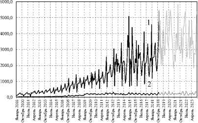
t , year

Source: own calculations.

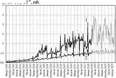
Figure 9. Investment dynamics in the UR healthcare in 2000–2018 and their forecast in 2019–2023: budget (1), private (2)

Р 2 ·10

-6

G 2 ·10 6000,0

5000,0

4000,0

3000,0

2000,0

1000,0

t , year

Source: own calculations.

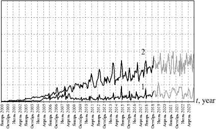
Figure 10. Investment dynamics in the UR culture in 2000–2018 and their forecast in 2019–2023: budget (1), private (2)

G 3 ·10^-6 , Р 3 ·10^-6, rub.

6000,0

5000,0

4000,0

3000,0

2000,0

1000,0

0,0

Source: own calculations.

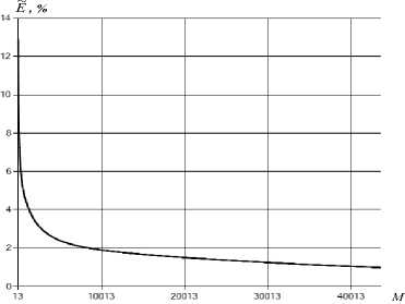
Figure 11. Dependence of the neural network training quality indicator on the number of iterations

Source: own calculations.

Source: own calculations.

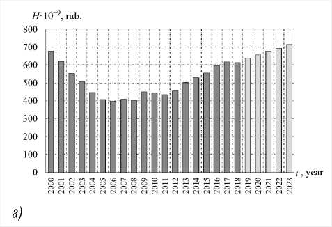
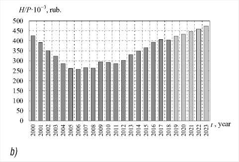
Figure 12. Human capital dynamics (a) and specific value of UR human capital (b) for 2000–2018 and its forecast in comparable prices

Figures 8–10 show the results of forecasting investments in the social sph ere of UR for the period 2019–2023. Figure 11 shows a graph of convergence to the 1% error level.

Deviation of pattern investment values from actual UR data for the period of 2000–2018 in health care is 1.4%, in education – 1.2%, in culture – 1.1%.

Based on the formula (10), the value of the HC UR for the period of 2000–2018 has been calculated. Figure 12 shows the results of calculating the HC value for the period of 2000–2018 and the results of the problem solving of predicting the size and dynamics of the HC using the results of problem solving of predicting the volume of investments in the HC based on neural network modeling for the period of 2019–2023.

Conclusion

We have built a neural network algorithm, on the basis of which the forecasting human capital problem was solved on the example of the socio-economic system of the Udmurt Republic.

Neural network modeling of predicted values of investment volumes in human capital has shown its effectiveness. Thus, the deviation of the pattern values of investments in the components of the HC UR from the actual data for the period 2000 – 2018 amounted to 1.4%.

Calculations showed that the human capital value of the Udmurt Republic decreased in the 2000 – 2006 interval, and then there was an increase in this indicator. The studied indicator has been showing the highest growth rates since 2013, and its further growth is predicted. In 2018, the human capital value per one UR resident amounted to about 400 thousand rubles.

The results obtained qualitatively correlate with the dynamics of changes in the human development index of Russia, determined by the UN experts which in the period from 2000 to 2012 increased from 0.71 to 0.79, and subsequently, until 2017, remained almost constant to a value of 0.80.

The Udmurt Republic is a Russia’s typical region in many socio-economic indicators ² . It is characterized by the average Russian values of these indicators. Therefore, the results and conclusions obtained during the research can be extrapolated to the RF as a whole.

The proposed methodology for calculating and forecasting the value, structure and dynamics of human capital can be used in assessing and comparing the socio-economic situation of the regions of the Russian Federation.

Список литературы Neural network forecasting algorithm as a tool for assessing human capital trends of the socio-economic system

Mincer J. Investments in human capital and personal income distribution. Journal of Political Economy, 1958, vol. LXVI, no. 4, pp. 281–302.
Schulz T. Investment in human capital. American Economic Review. 1961, vol. 51, no. 1, pp. 1–17.
Becker G.S. Investment in human capital: A theoretical analysis. Journal of Political Economy, 1962, vol. 70, no. 5, pp. 9–49.
Kuznets S. Quantitative aspects of the economic growth of nations. VIII: Distribution of income by size. Economic Development and Cultural Change, 1963, vol. 11, no. 2, part 2, pp. 1–80.
Ehrenberg R.G., Smith R.S. Sovremennaya ekonomika truda. Teoriya i gosudarstvennaya politika [Modern Labor Economics. Theory and Public Policy]. Moscow: MSU publishing, 1996. 198 p.
Koritskii A.V. Vvedenie v teoriyu chelovecheskogo kapitala [Introduction in the Theory of the Human Capital]. Novosibirsk: SibUPK publishing, 2000. 112 p.
Akopyan A.S., Bushuev V.V., Golubev V.S. Ergodynamic model of man and human capital. Obshchestvennye nauki i sovremennost’=Social Sciences and Contemporary World, 2002, no. 6, pp. 98–106 (in Russian).
Malkov S.Yu., Bolokhova K.A., Davydova O.I. Evaluation and prediction model of human capital development. Ekonomika i upravlenie: problemy, resheniya=Economics and management: problems, solutions, 2016, no. 7, pp. 7–16 (in Russian).
Aivazian S.A., Stepanov V.S., Kozlova M.I. Measuring the synthetic categories of quality of life in a region and identification of main trends to improve the social and economic policy (Samara region and its constituent territories). Prikladnaya ekonometrika=Applied Econometrics, 2006, no. 2, pp. 18–84 (in Russian).
Xu Y., Li A. The relationship between innovative human capital and interprovincial economic growth based on panel data model and spatial econometrics. Journal of computational and applied mathematics, 2020. DOI: 10.1016/j.cam.2019.112381
Timerbulatov R.M. Investment in human capital as a factor of improving company competitiveness. Vestnik Saratovskogo gosudarstvennogo sotsial’no-ekonomicheskogo universiteta=Vestnik of Saratov State Socio-Economic University, 2016, no. 1, pp. 40–42 (in Russian).
Kitaeva L.V., Khaibulaev Kh.U. Investments in human capital: problems of theory and practice. Vestnik ekspertnogo soveta=Expert Council Bulletin, 2018, no. 1–2 (12–13), pp. 93–100 (in Russian).
Chernov G.E., Chernova E.V. Human capital as a key vector of economic development in the XXI century. Obshchestvo: politika, ekonomika, pravo=Society: Politics, Economics, Law, 2016, no. 11, pp. 54–61 (in Russian).
Ryabykh V.N., Ryabykh E.B. The social- economic aspect of human capital in modern globalizing economy. Vestnik Tambovskogo universiteta. Seriya: Gumanitarnye nauki=Tambov University Review. Series: Humanities, 2015, no. 9 (149), pp. 129–136 (in Russian).
Serebryakova N.A., Volkova S.A., Shendrikova O.O., Volkova T.A. The role of human capital in the modern economy and indicators of its evaluation. Vestnik VGUIT=Proceedings of the Voronezh State University of Engineering Technologies, 2017, vol. 79, no. 4, pp. 253–259. DOI: 10.20914/2310-1202-2017-4-253-259 (in Russian).
Mikhaleva O.M. The role of human capital in the innovative development of territories. Vestnik Bryanskogo gosudarstvennogo universiteta=The Bryansk State University Herald, 2019, no. 1, pp. 183–189 (in Russian).
Stabinskaite Yu.A. The human capital rationale behind the economic growth of the European Union countries: application of the advanced methods to enhance an efficiency of national human capital stocks. Vestnik Rossiiskogo universiteta druzhby narodov. Seriya: Ekonomika=RUDN Journal of Economics, 2019, vol. 27, no. 1, pp. 35–48. DOI: 10.22363/2313-2329-2019-27-1-35-48 (in Russian).
Ketova K.V. Matematicheskie modeli ekonomicheskoi dinamiki: monografiya [Mathematical Models of Economic Dynamics: Monograph]. Izhevsk: IzhGTU, 2013. 284 p.
Schmidhuber J. Deep learning in neural networks: An overview. Neural Networks, 2015, vol. 61, pp. 85–117. DOI: 10.1016/j.neunet.2014.09.003
Nguyen G., Dlugolinsky S., Bobk M. Machine Learning and Deep Learning frameworks and libraries for large-scale data mining: A survey. Artificial Intelligence Review, 2019, vol. 52, pp. 77–124. DOI: 10.1007/s10462-018-09679-z
Vavilova D.D., Ketova K.V., Kasatkina E.V. Application of genetic algorithm for adjusting the structure of multilayered neural network for prediction of investment processes. In: Materialy VIII Mezhdunarodnoi konferentsii «Tekhnicheskie universitety: integratsiya s evropeiskimi i mirovymi sistemami obrazovaniya» [Proceedings of the VIIII International Conference "Technical Universities: Integration with European and World Education Systems"]. 2019, vol. 1, pp. 223–233 (in Russian).
Tsoy Yu.R., Spitsyn V.G. Evolutionary approach to design and training of artificial neural networks. Neiroinformatika=Neuroformatics, 2006, vol. 1, no. 1, pp. 34–61 (in Russian).
Yasnitskii L.N. Intellektual’nye informatsionnye tekhnologii i sistemy [Intelligent Information Technologies and Systems]. Perm: Perm State University, 2007. 271 p.
Effati S., Nazemi A. Neural network models and its application for solving linear and quadratic programming problems. Applied Mathematics and Computation, 2006, vol. 172, no. 1, pp. 305–331. DOI: 10.1016/j.amc.2005.02.005
Ghanbarzadeh M., Aminghafari M. A novel wavelet artificial neural networks method to predict nonstationary time series. Communications in Statistics-Theory and Methods, 2018, vol. 49, no. 4, pp. 864–878. DOI: 10.1080/03610926.2018.1549259
McCulloch W.S., Pitts W. A logical calculus of the ideas immanent in nervous activity. Bull. Math. Biophys., 1943, vol. 5, pp. 115–133.
Hebb D.O. The Organization of Behavior: A Neuropsychological Theory. Wiley, 1949. 335 p.
Rosenblatt F. Principles of Neurodynamics: Perceptrons and the Theory of Brain Mechanisms. Washington, D.C. Spartan books, 1962. 480 p.
Kohonen T. Self-Organizing Maps (Third Extended Edition). New York, 2001. 501 p.
Grossberg S. Competitive learning: From interactive activation to adaptive resonance. Cognitive Science, 1987, vol. 11, no. 1, pp. 23–63.
Werbos P.J. Beyond regression: New tools for prediction and analysis in the behavioral sciences. Harvard University, Cambridge, 1974.
Minsky M.L., Papert S. Perceptrons: An Introduction to Computational Geometry. Cambridge, Mass., 1969. 112 p.
Fukushima К., Miyake S., Takayuki I. Neocognitron: A neural network model for a mechanism of visual pattern recognition. IEEE Transaction on Systems, Man and Cybernetics SMC, 1983, vol. 13(5), pp. 26–34.
Hopfield J.J., Tank D.W. Neural computation of decisions in optimization problems. Biological Cybernetics, 1985, vol. 52, no. 3, pp. 141–152.
Haykin S. Neural Networks: A Comprehensive Foundation. United States, 1998. 842 p.
Hecht-Nielsen R. Confabulation Theory. Springer-Verlag: Berlin, Heidelberg, 2007. 116 р.
Yunusova L.R., Magsumova A.R. Algorithms for learning artificial neural networks. Problemy nauki=Science Problems, 2019, pp. 21–25 (in Russian).
Mitinskaya A.N., Matych M.A. Research of the forecasting problem using neural networks. Aktual’nye napravleniya nauchnykh issledovanii XXI veka: teoriya i praktika=Actual Directions of Scientific Researches of the XXI Century: Theory and Practice, 2015, vol. 3, no. 7-2 (18-2), pp. 30–31. DOI: 10.12737/15021 (in Russian).
Shagalova P.A. Implementation of the pattern recognition system for time series analysis based on the artificial neural network. Trudy Nizhegorodskogo gosudarstvennogo tekhnicheskogo universiteta im. R.E. Alekseeva=Transactions of NNSTU n.a. R.Е. Alekseev, 2015, no. 3(110), pp. 85–90 (in Russian).
Cavarretta F., Naldi G. Mathematical study of a nonlinear neuron model with active dendrites. Aims Mathematics, vol. 4, no. 3, pp. 831–846. DOI: 10.3934/math.2019.3.831
Aivazian S.A., Afanas’ev M.Yu., Kudrov A.V. Indicators of the main directions of socio-economic development in the space of characteristics of regional differentiation. Prikladnaya ekonometrika=Applied Econometrics, 2019, no. 2 (54), pp. 51–62 (in Russian).
Ketova K.V., Rusyak I.G., Romanovskii Yu.M. Mathematical modeling of the human capital dynamic. Komp’yuternye issledovaniya i modelirovanie=Computer Research and Modeling, 2019, vol. 11, no. 2, pp. 329–342. DOI: 10.20537/2076-7633-2019-11-2-329-342 (in Russian).
Rusyak I.G., Ketova K.V. Identification and forecast of generalized indicators of regional economic system development. Prikladnaya ekonometrika=Applied Econometrics, 2009, no. 3 (15), pp. 56–71 (in Russian).
Rutkovskaya D., Pilin’skii M., Rutkovskii L. Neironnye seti. geneticheskie algoritmy i nechetkie sistemy [Neural Networks. Genetic Algorithms and Fuzzy Systems]. Moscow: Goryachaya liniya – Telekom, 2006.

Еще

Статья научная