New exact solutions which describe 2-dimensional velocity field for Prandtl’s solution

The 2-dimensional ideal plasticity equations in case of steady-state problem have the form:

5а Г59        59 .)

2 k I —cos29+--sin29 | = 0,

5x     (5x        5yJ

— -2 k I— sin29- —cos29^ = 0,(1)

5y     (5x        5yJ

Г 5v   5v )       Г 5v   5v)

I +      I tg2 9 + l            ^y- | = 0,

(5 y   5x J       (5 x5y

^^Vy = 0,

5x5y here a is hydrostatic pressure, 9 is the angle between the first principal direction of stress tensor and axis Ox, k is plasticity constant, vxvy are components of velocity vector of strain field.

Prandtl’s solution is one of the practically applied and frequently used in different computations. This solution describes in particular the pressing of a thin layer of plastic material between two parallel stiff and rough plates, and it has the following form:

ax =-P - k(x - 2V1 - У2), ay =-p - kx, t = ky,               (3)

p is an arbitrary constant.

It is well known that to describe the plasticity state of material completely one should know velocity field.

Let’s substitute the equations (2) into the system (1). We get:

Г5vx  5v ) г----. VVx yl              I = Ji - У21+ I

(5x   5y J (5y5

here a , в , C , , C ₂ are arbitrary constants (if a = 0 Nadai’s solution comes out).

Let’s point out others solutions of the system (4). Notice that in variables ^ , n , where a = k (^ + n ) , 2 9 = ^ - n , the equations (2) are written as follows (5):

5 v, x di

5 v_x      5 v„         5v

- tg 9 -УУ = 0, -УУ + ctg 9 — x- = 0.

5i     5n       5n

If we put new variables into (5) using the formulas:

vx = u cos 9-v sin 9, vy = u sin 9 + v cos 9,                (6)

we’ll get a system (7):

5 v

5i

1 n 5 u   1 a

—u = 0,--- v = 0.

2 5n 2

Further we use the following procedure: we solve the system (7), put expressions from Prandtl’s solution for i and П into this system, make substitution (6) and find a velocity field which corresponds to the solution (3).

Let’s do it, for example, using the simplest solution of the system (7). It is obvious that

v = u

= exp2 ( i + n )

is a solution of the equations (7). Put it into the (6). We get: v_x = ( cos 9- sin 9 ) exp2 ( i + n ) , v_y = ( cos 9 + sin 9 ) exp2 ( i + n ) .

From Prantl’s solution (3) one can get easily

5 v   5 v y

—- + —- = 0.

5 x   5 y

i + n =--- x - sin 2 9 , cos 2 9 = y . k

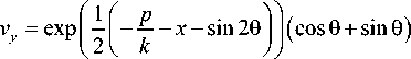
And finally we find a new velocity field:

One can see that because of its linearity the system (4) has an infinite set of solutions which can be used for the

Г 1 Г P v, = exp —-- ^x ( 2 ( k

analysis of the stress-strained state of a plastic medium.

At the present moment two classes of solutions of this system are known, Nadai’s solution [1] and Ivlev–Senashov’s solution [2], which are the following:

v_x = -a xy + в x - a arcsin y -

- x - sin 2 9 | I ( cos 9- sin 9 ) ,

-a y>] 1 - y ² - 2в1 - y ² + C 1, _ Г x ² y ²)

^Vy = ^al T⁺т!^{-в y +} C 2 ,

By using this scheme some other velocity fields are found.

For the equations (7) solutions are given in [3]. Further with respect to these indicated solutions, 5 more classes of new solutions of the equations (5) are built.

f. i+n) u = cos Л----

( 2 J

Г i-n1     . Г E-n1

A cos ц---- + B sin ц---- .

(     2 J (     2 J

*The work was carried out with support from FOP “Scientific and Scientific-Pedagogical Personnel of Innovative Russia” for 2009–2013 years.

Mathematics, mechanics, computer science

Here A , B , ц, X are arbitrary constants; ц² -X² = 1.

In this case

5 u     X . ( E + ni

— = — sin I X---- | x

I. E+n

3) u = exp I X 2

I E-ni       I E-n

A cos ц---- + B sin ----

Г 2 J      I 2

dp 2

Here A , B , ц, X are arbitrary constants; ц² + X² = 1.

In this case

. I E-ni n ■ I E-n x A cos ц---- + B sin ц----

I 2 J I 2

ц U E+n

+—cos X----

2 I 2

. ■ I E-n A sin ц----

I 2

I E-ni

B cos ц----- .

I 2 J

From the equations (7) we get

JE + n v = -X sin X----

I 2

Ii E+n +ц cos X----

I 2

. L E + n v = X exp IX ——

f. E+n

+ ц exp IX 2

, I E-n i „ ■ I E-n A cos ц  + B sin ц

(     2 J (     2

. • I E-n

A sin ц----

I 2

I E-n 1

B cos ц----- .

I 2 J

. I E-n 1 I E-n

A cos ц---- + B sin ц----

(     2 J (     2

I X[ p                  11

v, = exp — \ -—-x-sin20 x x I 21 k             JJ

-. । E-n A sin ц----

Г 2

I E-n i

B cos ц----- .

(     2 J

x[ A cos ( ц0 ) - B sin ( p0 ) ] cos 0-

li I XI P ■     ) I

- -X exp — \--- x - sin2 0 x

I I 2 1 k               JJ

Making substitution for u , v into the equations (6) and

E-n taking into account the equalities (8) and 0 = 2   we get

x[ A cos ( ц0 ) - B sin ( p0 ) ]

+ц exp X

v x = cos 1 2 1 - ^p - x - sin 2 0 J J[ A cos ( ц0 ) - B sin ( p0 ) ] cos 0-

-1 -X sin 121 - ^p - x - sin 2 0 J J [ A cos ( ц0 ) - B sin ( p0 ) ] +

+ц cos 1 2 1 - ^p - x - sin2 0J J[- A sin ( ц0 ) - B cos ( p0 ) ] J sin 0 ,

v_y = cos 121 - k - x - sin2 0J J[ A cos ( ц0 ) - B sin ( p0 ) ] sin 0 +

IX

-X sin —

I 2

-

^p k

-

x - sin 20 I J[ A cos ( ц0 ) - B sin ( ц6 ) ] +

I X +ц exp I —

px

2 k 2

^{1 -} У y

[- A sin ( ц0 ) - B cos ( p0 ) ] sin 0 ,

I XI p v, = exp — — ^y I 2 1 k

- -

sin2 0 I Ix

x[ A cos ( ц0 ) - B sin ( ц0 ) ] sin 0 +

L IXI p . „Ji + X exp — \--- x - sin2 0 x

I      ^r I 2 1 k J J

x [ A cos ( ц0 ) - B sin ( ц0 ) ] +

( ц0 ) ] I cos 0.

+ ц cos I 21- ^p - x - sin 2 0 J![- A sin ( ц0 ) - B cos ( ц0 ) ] I cos 0.

I„E+n । в I E-ni „ IE-ni 4) u = exp IX 2 I A exp 1ц 2 I + B exp I 2 I •

E + n

Il E + n

2) u = sin X-----

I 2

I E - n । I E - n

A cos ц---- + B sin ----

I 2 J I 2

Here A , B , ц , X are arbitrary constants; X² -ц² = 1.

In this case

Here A , B , ц , X are arbitrary constants; ц² -X² = 1.

In this case

. L E + n 1 v = X exp X---- x

I 2 J

. L E + n v =-X cos X----

I 2

■ U E + n + ц sin X----

I 2

And

, Г E-ni „ . I E-n

A cos ц---- + B sin ц----

I 2 J I 2

I E-n

A sin ц---- (     2

i E-ni

B cos ц----- .

(     2 J

v x = sin 121- ^p - x - sin 2 0J J [ A cos ( ц0 ) - B sin ( p0 ) ] cos 0- ,

-1 -X cos 1 2 1 - ^p - x - sin 2 0J J [ A cos ( ц0 ) - B sin ( p0 ) ] +

+ ц sin 1 2 1 - p - x - sin 2 0 J J [- A sin ( ц0 ) - B cos ( ц0 ) ] j sin 0 ,

I Xi p _„iir vy = sin I 21 -k ~ x - sin 20J![ A cos (ц0)- B sin (ц0)] sin 0 +

IX + X cos — I 1 2

p

k

x - sin2 0 | I[ A cos ( ц0 ) - B sin ( p0 ) ] +

+ ц sin I 21- ^p - x - sin2 0J J[- A sin ( ц0 ) - B cos ( ц0 ) ] I cos 0.

. I E-ni n I E-n x A exp 1ц —— I + B exp 1ц 2

Г. E + n 1

+ ц exp X---- x

I 2 J

. I E-ni n I E-ni x - A exp 1ц 2 I + B exp 1ц 2 I •

I XI p . li v = exp —---x - sin20 x x

1 2 1 k           JJ

x[ A exp ( -ц0 ) + B exp ( -ц0 ) ] cos 0-

x - sin 2 0 | |x

x[ A exp ( -ц0 ) + B exp ( -Ц0 ) ]

+ц exp 121- p - x - sin 2 0J J [- A exp ( -ц0 ) + B exp ( -ц0Ш sin 0 ,

I X ^v y = exp I 2

p

k

- Y -

sin 2 0 I Ix

x [ A exp ( -Ц0 ) + B exp ( -Ц0 ) ] sin 0 +

^p k

I X I P                    i lr v = exp — -—-x - sin29 [-A 9 + Bl sin 9 + y V 2 V k            Л[        ]

х[ A exp ( -ц9 ) + B exp ( -ц9 ) ] +

I Xf P +ц exp l -I -^

V 2 V k

- x - sin2 9 I l[- A exp ( -ц9 ) + B exp ( -ц9 ) ] I cos 9 .

f\ -+n

5) u = exp IX 2

AB\

Here A , B , X are arbitrary constants; X ² = 1.

In this case

v = X exp (х ^ ^{+ П} ) A ^-—^П + B - A exp fx^-^^ .

V 2 JL 2       ] I 2 J

I X I P            _„i ir v, = exp — -—-x - sin29 [-A 9 + Bl cos 9

^x V 2 V k            Jr         ^]

p

k

- x - sin2 9 I l [ - A 9 + B ] -

[.      f X f p

+ X exp

I        V 2 V k

- x - sin2 9 | l [ - A 9 + B ] -

- x - sin2 9 I I I cos 9 .