New Mean-Variance Gamma Method for Automatic Gamma Correction

Author: Meriama Mahamdioua, Mohamed Benmohammed
Journal: International Journal of Image, Graphics and Signal Processing(IJIGSP) @ijigsp
Article in issue: 3 vol.9, 2017.
Free access
Gamma correction is an interesting method for improving image quality in uncontrolled illumination conditions case. This paper presents a new technique called Mean-Variance Gamma (MV-Gamma), which is used for estimating automatically the amount of gamma correction, in the absence of any information about environmental light and imaging device. First, we valued every row and column of image pixels matrix as a random variable, where we can calculate a feature vector of means/variances of image rows and columns. After that, we applied a range of inverse gamma values on the input image, and we calculated the feature vector, for each inverse gamma value, to compare it with the target one defined from statistics of good-light images. The inverse gamma value which gave a minimum Euclidean distance between the image feature vector and the target one was selected. Experiments results, on various test images, confirmed the superiority of the proposed method compared with existing tested ones.
Gamma value estimation, Correction of gamma, Improving image quality, Mean, Variance
Short address: https://sciup.org/15014172
IDR: 15014172
Text of the scientific article New Mean-Variance Gamma Method for Automatic Gamma Correction
Published Online March 2017 in MECS
The uneven luminance is one factor which directly reduces the appearance of an image and decreases the effectiveness of many artificial systems. For example, in face recognition, the changes in illumination affect dramatically the performance of recognition systems, because different lighting conditions can lead to very different images of the same person. The image with low contrast also comes from using poor quality imaging devices, that having bad characteristics and exploited by a poorly trained operator, and more, many devices used for capturing, printing or displaying the images generally apply a non-linear effect on luminance [1-3]. Given this, the application of a pretreatment method that is able to overcome these problems is a crucial need for any image processing system.
Increasing the contrast and adjusting the brightness are the basis of image quality enhancement algorithms [4]. Most commonly, contrast enhancement based on histogram equalization (HE) has achieved more attention from researchers due to its simplicity, effectiveness and its property of redistribution of intensity values of an input image [1, 5]. However, sometimes the original HE cannot give satisfying amelioration and dramatically changes the average brightness of the image [6]. Various methods have been published to limit the inadequate improvement in HE [6], such as Brightness preserving Bi-Histogram Equalization (BBHE), Dualistic Sub-image Histogram Equalization (DSIHE), Minimum Mean Brightness Error Bi-Histogram Equalization (MMBEBHE) and Recursive Mean-Separate Histogram Equalization (RMSHE). In BBHE and according to the mean intensity, two separate histograms from the same image were formed and then equalized independently, where for DSIHE, the median gray intensity was used to split the histogram into two separate histograms. Although DSIHE can maintain better the brightness and entropy, both of DSIHE and BBHE cannot adjust the level of enhancement and are not robust to noise [6]. MMBEBHE is an extension of BBHE, which offers maximum brightness preservation better than BBHE and DSIHE [6]. It based on the separation of the histogram into two sub-parts using threshold level. RMSHE is a generalization of BBHE technique where the segmentation was done more than once and recursively, and the mean brightness of the output image converges to the mean brightness of the input image as the histogram segmentation increases [7].
Another technique which is often used to adjust the contrast of images is gamma correction. It is generally used to counter the power-law effect of the imaging device. It is defined by Vout = VinY expression, where Vtn is the intensity at one pixel location in the input image, Vout is the transformed pixel intensity and у is a positive constant. If the gamma value у is known, we can inverse this process by using Vn = Vou1 1 /Y expression.
The value of gamma used modifies the pixels intensity to appropriately enhance the image. This value of gamma is typically determined experimentally by passing a calibration target with a full range of known luminance values through the imaging system [8]. However, it is often difficult to select suitable gamma-value without the knowledge about the imaging device. Moreover, the inadequate environment lighting conditions contribute to the cause of low contrast. So, the value of gamma is to be chosen in such a way that all these factors are together taken into consideration [3].
Recently, some algorithms have been developed to determinate the gamma values automatically for offline images, as methods proposed in [2-3, 8-11].
In [8], a blind inverse gamma correction technique had been developed. The approach exploited the fact that gamma correction introduces specific higher-order correlations in the frequency domain. These correlations can be detected using tools from the polyspectral analysis. The value of gamma was then estimated by minimizing these correlations by applying a range of gamma values between 0.1 and 3.8 .
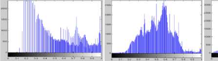
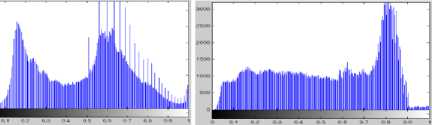
The authors in [2] had applied a range between 0.1 and 3 in increments of 0.1 of inverse gamma value to a given image, and had computed texture mask of each image, then they had summed up the values of each texture mask to select the gamma value that had maximum summation.
The basic idea for method proposed in [10] is that the homogeneity value - which can be calculated by cooccurrence matrix- in an image not suffering from gamma deformation, has a lower value (near to zero). The gamma value was then estimated locally by minimizing these homogeneities. First, for local gamma correction, the image was divided into overlapping windows, and then the authors had applied a range of inverse gamma values from 0.2 to 2.2 with 0.1 step to each window. By extracting the homogeneity feature from the cooccurrence matrix of the window, the gamma value associated with the minimum homogeneity was then considered as the best gamma value for enhancement.
In [9], an adaptive gamma correction method based on gamma correction function was proposed, where a mapping between pixel and gamma values was built. The gamma values were then revised using two nonlinear functions to prevent the distortion of the image.
The enhancement method proposed in [11] was based on local gamma correction with level thresholding. Three level thresholds were used to segment the image into three gray levels on the basis of maximum fuzzy entropy. Local gamma correction was then applied to these three levels.
The authors in [3] proposed to use fuzzy theory to estimate the exposure level of the input image. They had first assessed the level of exposure in the input image using several fuzzy rules. In the second stage, they had derived the gamma value as a function of the exposure level.
By comparing histogram equalization techniques and gamma correction method to overcome the effects of light, the gamma correction is more advantageous [9]. However, the existing methods don’t assure that the corrected images result have statistics similar to images free from gamma distortion.
Taken into consideration the previous discussion, we aim in this paper to overcome the problem of low light and low contrast of images by proposing a simple and effective automatic gamma correction method. Our proposed MV-Gamma method estimates the amount of gamma automatically without any prior information about the environmental illumination and the imaging device. Basing only on image’s mean and variance values, the present method tried to change the statistics (mean and variance) of the damaged image to be as close as possible to those of images with good illumination, by comparing a feature vector of means/variances of damaged image to a target vector resulting from correctly-exposed images.
The rest of this paper is organized as follows: Section II explains the principle of gamma correction. Section III is devoted to illustrating proprieties of images with good quality. The evaluations techniques of enhancement methods are presented in Section IV. Our proposition is presented in Section V. In Section VI, we discuss the comparative results. Finally, Section VII concludes this work.
-
II. Gamma Correction
Gamma correction is essentially a gray-level transformation function applied on images to enhance their imperfect luminance and to correct the power-law effect of the imaging device. This later is measured by function given in (1) [21]:
Vout = с Ц/ (1)
where Vln E [0,1] denotes the input image pixel intensity , V0ut is the transformed pixel intensity, c and у are positive constants. For simplicity, c is often taken to be unity.
Reversing this process is possible if the gamma value is known [8], by using function (2)
Vm = V0J (2)
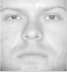
Fig. 1 a shows an image with three different gamma values. It can be seen from this figure when the amount of у is less than one, the transformed image becomes lighter than the original image and its histogram is shifted to the right side. In addition, when the value of is greater than one, the transformed image becomes darker than the original one and its histogram is shifted to left side.
Gamma correction is an interesting method for improving image quality. It can be used individually [2-3, 8-11], and as a step in others pretreatment methods like in [12-19, 29]. In the second hand, these enhancement methods are applied in different fields. In face recognition, the preprocessing step that corrects or eliminates the change of light is a crucial need for improving the performance of recognition system. So, find the adequate value of gamma automatically will improve greatly the results of preprocessing methods, which ameliorates the performance of recognition systems.
Our proposition is based on statistics (mean and variance) of good-light images to create the target vector feature. The good-light image histogram and statistics are discussed in the next Section.
-
III. Proprieties of Good Quality image (Histogram, Mean, and Variance)
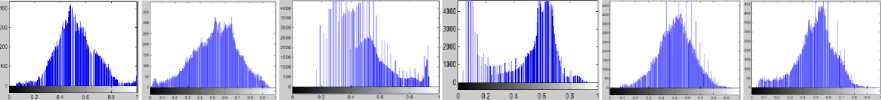
The histogram has been widely used to represent, analyze and characterize images. Histogram analysis shows that the under-exposed images have a histogram shifted to the left side, and over-exposed ones have a right-shifted histogram, where the correctly-exposed images have a histogram centered in the middle, as shown in Fig. 1.
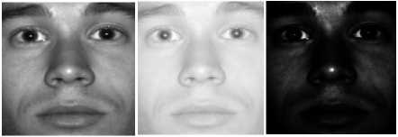
Gamma=1 Gamma=0.25 Gamma=4
(a.1) ( a.2) ( a.3)
Mean=0.4558
Variance=0.02286
Mean=0.8108
Variance=0.0064
Mean= 0.0726
Variance=0.0078
(b.1) (b.2) (b.3)
Fig.1. Application of different gamma values (a.1) - (a3) Image with various gamma values (b.1) - (b.3) Histograms and Images statistics
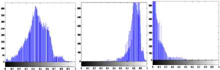
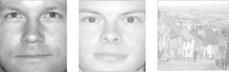
In addition, the correctly-exposed images have means intensities close to the median histogram value (~ 0.5 , when intensities values E [0,1]) and they have convergent and small variance values, as examples in Fig.2 shown.
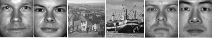
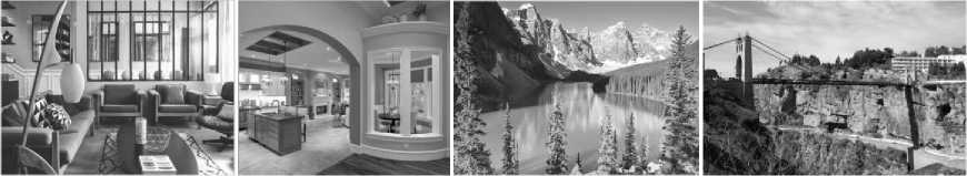
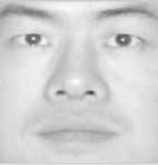
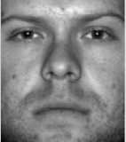
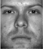
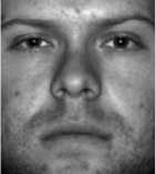
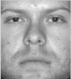
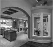
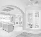
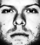
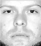
To calculate the target vector feature used in our method (see Section V), we calculate average means and average variances, noted Avg-means and Avg-vars resp., of a set of correctly-exposed images. This set composed from some properly-exposed natural images and a subset of S1 of Extend CroppedYale face database [26, 27], where the images of this later are taken under different illumination conditions and divided into 5 subsets according to the lighting angle. Subset S1 contains images captured in relatively good illumination conditions, while for the images of subsets labeled S2 to S5, the lighting conditions are going from good to worse.
The remaining details of our method are explained in Section V, but before, a set of techniques used to evaluate the enhancement methods are presented in the following Section.
-
IV. Performance Evaluation
To evaluate image enhancement methods, we can find in literature subjective and objective techniques. The subjective techniques based on human vision and his estimation of image quality. However, the objective ones based on numerical evaluation by using evaluation of histogram and/or using quality factors (separately or together) as:
Mean = 0.5072
Variance = 0.0295
Mean=0.5258
Variance= 0.0306
Mean=0.5050
Variance =0.0392
Mean=0.5165
Variance= 0.0211
Mean=0.4558
Variance=0.0228
Fig.2. Examples of correctly-exposed images
-
- PSNR (Peak Signal-to-Noise Ratio)
-
- AMBE (Absolute Mean Brightness Error)
-
- SSIM (Structure Similarity Index
We give in following lines the numerical evaluation factors formulas used in this paper [7, 22-25].
-
A. Peak Signal to Noise Ratio (PSNR)
MSE (Mean Squared Error) is calculated through (3), where N is the total number of pixels in the input image X = {хц } or output image Y = { У г,;- }. Based on MSE, we calculate PSNR defined by (4). According to the definition of PSNR, the output image quality is better if image has maximum PSNR.
MSE = ^ (xi: J У1^2(3)
N
PSNR = 10 log, 0-^-(4)
where d is the maximum possible value of a pixel.
-
B. Absolute Mean Brightness Error (AMBE)
AMBE determines the error value between the two compared images. Suppose XM is the mean of the input image = { Хц^ , and MM is the mean of the output image M = { y ,; }.
The AMBE is calculated through (5)
A MBE (X,M)=X m -M m (5)
Minimum AMBE is obtained when output image has an almost same mean as the input image mean.
-
C. Structure Similarity Index (SSIM )
SSIM is used for calculating the similarity between two images. The value of SSIM varies in between -1 and 1.
(2 Vy+C i )(2 aXY +c 2 ) (А +м ) + c l )( °x +2y + 2 ) )
Ci = (^L )2(7)
C2 = ( k2L)2(8)
where L is a dynamic range of pixel value, and default values of k 1 and k 2 are {k 1 , k 2 } = {0.01 , 0.03}.
There is no universal quality factor to estimate the quality of enhanced image. In the Experimental Section, and to evaluate our proposed method, we used the subject method and all cited evaluation factors to prove the superiority of our proposed approach. But before presenting these results, we explain our proposed method details in the following Section.
-
V. Proposed Method
In our proposition, the image rows and columns are valued as a random variable like in [20], where we can calculate a feature vector of means/variances of image rows and columns. In the other hand, we analyzed images taken in good lighting conditions to find the adequate mean and variance values. These values are used to compose a target feature vector. After that, we apply a range of inverse gamma values on the input image and calculate the feature vector of means/variances for each inverse gamma value. The inverse gamma value which gives a minimum Euclidean distance between its related feature vector and the target one is selected.
More details on the principle, steps and defaults values of the proposed method are discussed in the following lines.
-
A. Method principle
Basing on the idea presented in [20], where the image is considered as a matrix and every row and column is numerically valued as a random variable, we can calculate for each one its mean and variance to construct a feature vector. The examination of image row by row and column by column allows us to benefit from the advantages of part-by-part image processing, where we can avail the details of the pixels intensities better than using the image in whole, and at the same time without examining them one by one.
The goal of this proposal was to enhance the low light and low contrast image by mapping its mean and variance to be similar as possible to these of the image taken under good lighting conditions, all by changing the values of the mean/variance of each row and column. However, and relative to the spatial distribution of objects in the image, the means/variances vector values have not taken exactly the same target values, but they become as close as possible, and as a result, mean and variance values for the whole enhanced image are really improved as we can see later in this paper.
-
B. Steps of proposed method
The key steps for our proposed method are as follows:
-
1. First, we use the average means and average variances values of images taken in good lighting conditions to construct a target vector (see Section III). For image with (r * c) size, the target vector composes of (r+c) Avg-means and (r+c) Avg-vars values ( 2*(r+c) in total), as shown by Fig. 3.
-
2. Then, for each damaged image, we estimate the gamma value by applying a range of inverse gamma values [ aa Z1,vaZ2] in increments of Step, , and we calculate for each inverse gamma value the means/variances feature vector, where the first (r + c) elements are the means of lines and columns of the image and the last (r + c) are the variances of rows and columns. The inverse gamma value which gave a minimum Euclidean distance between its related feature vector and the target one is selected.
-
C. Settings of parameters
For achieving the presentation of our MV-Gamma method proposed in this paper, we need to set their parameters related to the target vector and the interval of gamma used.
-
• Target vector values
The target vector is composed of average means/variances values of correctly-exposed images. By using the method explained in Section III, we found ( Avg-means, Avg-vars) ~ (0.5077, 0.0268). The target vector feature formed by these values is the one used for all type of images presented in the rest of this paper.
-
• Gamma range parameters
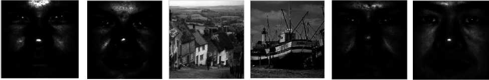
For gamma range, we have applied two ranges of inverse gamma values with two different increments according to the input image state. We have used the mean of the input image to select the adequate interval as follows:
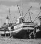
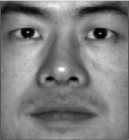
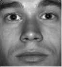
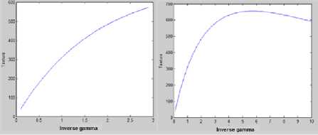
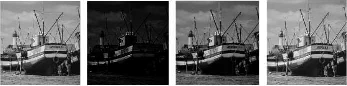
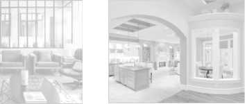
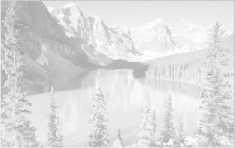
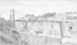
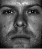
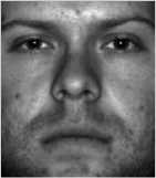
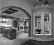
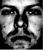
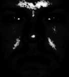
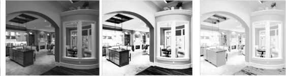
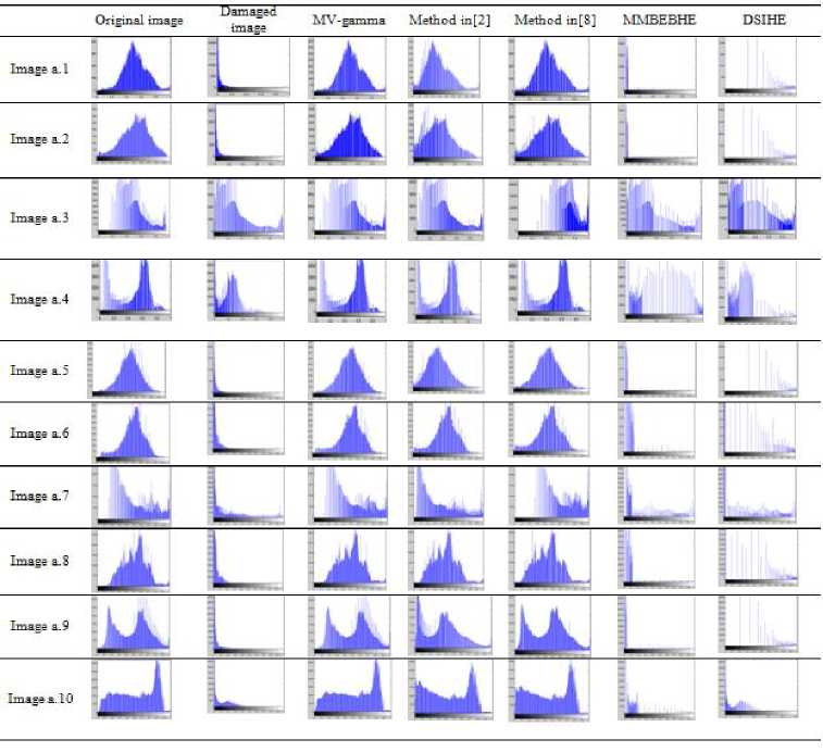
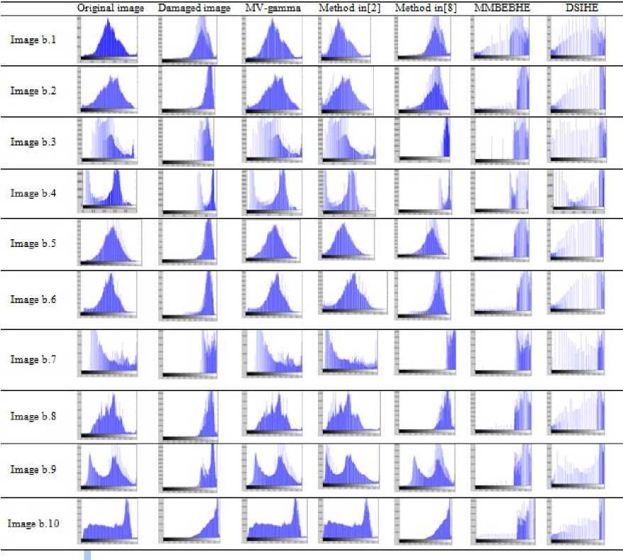
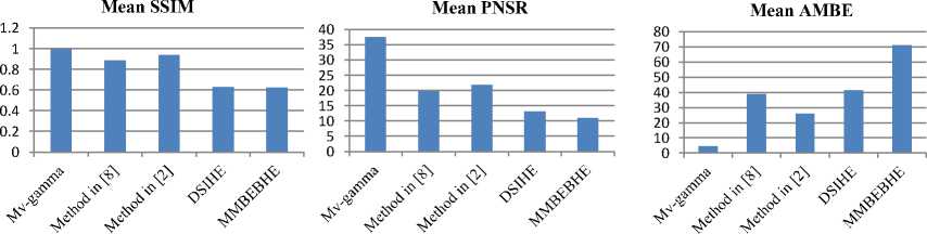
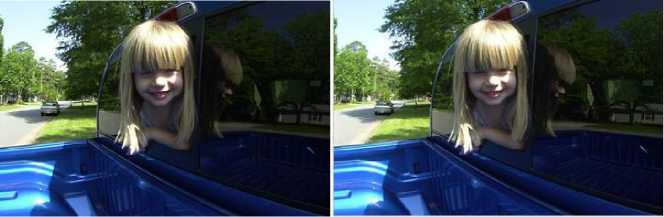
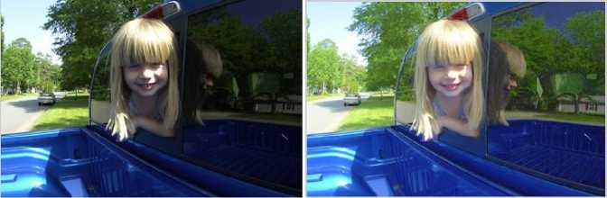
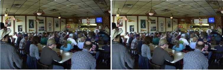
if 0 if 0.5 < mean tℎ en у 1 ∈]1, 10], witℎ step Step2 = 0.1 Fig.3. Feature vector (a) (b) Fig.4. Diagram of total texture mask values used in method [2] for the [0.1. .3] and [0.1. . 10] ranges, for the same image (a) Diagram of total texture mask for range [0.1, 3]. (b) Diagram of total texture mask for range [0.1, 10]. In reason to put the methods used in the experimental section in same conditions, we use the range of [0.1,10] for the compared gamma-estimation methods. This choice affects the tested methods as follows: - For the method proposed in [2], the gamma value used was the peak of image texture mask which can be schematized by a diagram as in Fig.4. In this method, the interval [0.1, 3] was used. This interval gave wrong values for strongly deformed images, where the value of inverse gamma found is not the peak of the diagram as the method assumed. As Fig.4 shown, the inverse gamma estimated for the range [0.1, 3] is 2.9 (Fig.4 a). When we use the [0.1, 10] range, the inverse gamma estimated is 5.8, and it is really the diagram peak (Fig.4 b). - The authors in [8] used [0.1, 3.8] range as the widest interval. By using [0.1, 10] interval, the results change and become best for dark images as Fig. 5 shown. In this figure, image improved by using [0.1, 10] range, has an SSIM closer to 1 than this of image improved by using [0.1, 3.8] interval. Moreover, mean found by applying the [0.1, 10] range is the nearest to the mean of the image with good quality. Our proposal approach is simple and effective. Its performance is proved in the next Section, where we evaluate it by using several techniques. VI. Experimental Results Our proposed method can be applied to improve various grayscale and color images. Its performances, using the subjective and the objective evaluations of images quality, were compared with those generated by the methods proposed in [2, 8] and two variants of histogram equalization methods, DSIHE and MMBEBHE. For that, we used Matlab environment to implement these methods, where we have based on the code proposed by the author in [28] for programming the method presented in [8]. To prove the effectiveness of our proposed method to restore different type of images, we choose for our experiment a set of images of different nature (varied between faces, natures, homes,...). It composed of some standard images, some Cropped Extend Yale database images, and other images taken from the web, as we can see in the rest of this Section. To be able to apply gamma correction, all the images used have intensities in [0, 1], which are needed to be normalized to [0, 255] intensities when calculating the quality factors. For grayscale images, our strategy is first to apply random gamma values on correctly-exposed images to compose two sets of damaged images (a set of light images and a set of dark images). Fig.6 shows ten correctly-exposed images used, where the dark and the light damaged versions are presented in Fig.7 and Fig.8 respectively. Their qualities compared to the original ones are evaluated by SSIM, PNSR, and AMBE as Table 1 and Table 2 illustrate. Then, we apply the five tested method to restore the damaged images and evaluate the resulted ones by comparing them to the original images, in terms of SSIM, PSNR, AMBE and their histograms. Examples of corrected images by the five tested methods, with their means and variances values, are given first in Fig 9. As we can see, our method gives images means and variances closer to those of correctly-exposed images ( (Mean, Variance) ≈ 0.5077, 0.0268)) (a) (b) (c) (d) Fig.5. Example of range changing effect for method proposed in [8] (a) Original image (b) Image damaged by a random value of gamma (c) Image improved by using [0.1,3.8] interval (SSIM=0.7898 and Mean=0.3137) (d) Image improved by using [0.1,10] interval (SSIM=0.9978 and Mean=0.5050) 1 2 3 4 5 6 7 8 9 10 Fig.6. Ten gray correctly-exposed images 1-10 Original images version a.1 a.2 a.3 a.4 a.5 a.6 a.7 a.8 a.9 a.10 Fig.7. Dark damaged images version of images presented in Fig.6. (a.1) - (a.10): dark damaged images b.1 b.2 b.3 b.4 b.5 b6 b.7 b.8 Fig.8. Light damaged images version of images presented in Fig.6. (b.1)- (b.10): light damaged images b.9 b.10 Table 1. Qualities estimation of dark damaged images compared to the original images. Images a.1 a.2 a.3 a.4 a.5 a.6 a.7 a.8 a.9 a.10 SSIM 0.0606 0.0618 0.7766 0.5033 0.0498 0.0971 0.3091 0.1108 0.0759 0.1906 PSNR 6.2391 5.7709 14.8604 9.7009 6.1334 6.6367 8.5624 6.2840 5.91249 6.6158 AMBE 119.68 125.48 44.19 79.010 121.7936 114.7266 89.3378 119.7555 119.6705 109.6093 Table 2. Qualities estimation of light damaged images compared to the original images. Images b.1 b.2 b.3 b.4 b.5 b.6 b.7 b.8 b.9 b.10 SSIM 0.8713 0.6686 0.6145 0.6659 0.7309 0.7382 0.5999 0.7515 0.6136 0.6404 PSNR 12.8746 8.6496 9.7332 8.4092 9.2724 9.1717 8.3639 9.5007 8.4502 8.55196 AMBE 56.1729 89.6932 97.0245 84.2163 85.3178 86.6178 87.8752 82.1935 89.6308 86.5533 The results found by applying the five tested methods to restore the tested images are given as SSIM in Table 3 (resp. Table 6), PNSR in Table 4 (resp. Table 7) and AMBE in Table 5 (resp. Table 8) for dark images (resp. for light images). For numerical evaluation, the proposed algorithm provides a better SSIM, PNSR, and AMBE values. Let us recall that (see section IV), the best value for SSIM is the closest to 1, for PNSR is the largest one and for AMBE is the smallest one. As we can see in Table 3 and Table 6, for our method and for the two cases (dark and light images), the value of SSIM > 0.99 (except for image a.3 its value is 0.9835, and for image b.3 it equals to 0.9855). The SSIM values are varied from one image to another for the others methods, from which SSIM can decrease to 0.7809 for the method proposed in [2] (image a.9), to 0.4600 for the method proposed in [8] (image b.7), to 0.3483 for the DSIHE method (image a.10) and down to 0.0690 for the MMBEBHE method (image a.2). The PNSR values (see Table 4 and Table 7) of our method are between 24.5724 and 49.4709, where for the others methods are as follow: 6.7047 ≤ PNSR ≤ 27.7050 for method proposed in [8], 8.7805 ≤ PNSR ≤ 29.8874 for method proposed in [2], 9.4251 ≤ PNSR ≤ 17.4724 for DSIHE method, 2.0069≤ PNSR ≤15.8525 for MMBEBH method The AMBE (see Table 5 and Table 8) for our method is < 8.8393 (except for image number four, where AMBE=14.5 for a.3 and 13.3912 for b.3). Its value reaches 102.3075 for method in [8] (image b.7), 47.3398 for method proposed in [2] (image a.9), 80.14 for DSIHE method (image a.4) and 117 for MMBEBHE (image a.2) This numerical evaluation indicates that the quality of the images restored by our method is the closest to the quality of the original images before their deformation. The histograms comparison confirms this result too, where images enhanced by our method have the most similar histograms to these of the original images, as Fig 10 (for dark images) and Fig 11 (for light images) shown. It means that our method restored the deformed images better than the others methods. a.5 b.5 a.8 b.8 MV-gamma Mean=0.5103 Variance=0.0212 Mean=0.5137 Variance= 0.0211 Mean=0.5045 Variance=0.0263 Mean=0.5095 Variance=0.0261 Method in [8] Mean=0.4540 Variance =0.0226 Mean= 0.6545 Variance = 0.0148 Mean=0.4341 Variance=0.0287 Mean=0.8294 Variance=0.0059 Method in [2] Mean=0.3410 Variance =0.0230 Mean=0.3976 Variance =0.0233 Mean=0.4324 Variance=0.0287 DSIHE Mean=0.3539 Variance =0.1082 Mean 0.6900 Variance= 0.0905 Mean=0.3064 Variance=0.1101 MMBEBHE Mean=0.0473 Variance =0.0203 Mean=0.8338 Variance = 0.0219 Mean=0.0781 Variance=0.0197 Mean=0.3805 Mean =0.6962 Mean 0.8338 Variance= 0.0296 Variance=0.0908 Variance= 0.0175 Fig.9. Examples of images corrected by the five methods with their means and variances Table 3. SSIM values of corrected dark-images (by the five methods) Images SSIM MV-gamma Method in [8] Method in [2] DSIHE MMBEBHE a.1 0.9980 0.9900 0.8960 0.4240 0.0750 a.2 0.9970 0.9800 0.8420 0.4045 0.0690 a.3 0.9835 0.8300 0.9655 0.7255 0.7736 a.4 0.9983 0.9765 0.9123 0.4991 0.4592 a.5 0.9986 0.9900 0.8993 0.4015 0.0583 a.6 0.9950 0.9900 0.9864 0.3035 0.1950 a.7 0.9995 0.9500 0.8167 0.4699 0.3747 a.8 0.9991 0.9700 0.9723 0.3965 0.1657 a.9 0.9981 0.9700 0.7809 0.4579 0.0983 a.10 0.9990 0.9600 0.9238 0.3483 0.1536 Table 4. PNSR values of corrected dark-images (by the five methods) Images PNSR MV-gamma Method in [8] Method in [2] DSIHE MMBEBHE a.1 37.6390 27.7050 16.1940 12.0600 6.7410 a.2 33.0178 23.1684 14.6367 11.3630 6.2694 a.3 24.5724 12.1502 22.7504 17.4724 15.8525 a.4 37.1965 23.3527 18.4908 9.4251 12.2041 a.5 37.1454 27.3060 16.0595 12.0472 6.5210 a.6 29.0800 24.6731 24.5553 9.8324 6.9730 a.7 49.4709 19.3295 15.4223 11.1996 9.6305 a.8 38.4200 21.5277 21.3672 10.7941 6.8673 a.9 36.3822 22.7796 14.3620 11.86400 6.4474 a.10 44.7101 23.7311 20.58931 10.40852 6.7695 Table 5. AMBE values of corrected dark-images (by the five methods) Images AMBE MV-gamma Method in [8] Method in [2] DSIHE MMBEBHE a.1 3.2000 10.3300 39.0000 41.6700 112.1000 a.2 5.5500 17.3700 46.5000 51.0000 117.0000 a.3 14.5000 59.9900 17.9100 22.1400 38.0000 a.4 3.4800 17.0361 29.9100 80.1400 43.1200 a.5 3.4813 10.8638 39.7646 36.8762 115.1128 a.6 8.8393 14.7002 14.9028 60.0561 109.8835 a.7 0.7345 25.6264 41.1051 63.2490 77.0732 a.8 2.9964 21.0827 21.4787 53.2709 111.5765 a.9 3.7298 17.9823 47.3398 51.0386 110.8697 a.10 1.3620 15.8815 22.8232 64.2646 105.0184 Fig.10. Histograms comparison for corrected-dark images by the five methods Table 6. SSIM values of corrected light-images (by the five methods) Images SSIM MV-gamma Method in [8] Method in [2] DSIHE MMBEBHE b.1 0.9993 0.8900 0.9503 0.7233 0.7843 b.2 0.9996 0.9200 0.9403 0.7175 0.7228 b.3 0.9855 0.5100 0.9793 0.7579 0.7447 b.4 0.9976 0.5800 0.8858 0.8226 0.7453 b.5 0.9986 0.9300 0.9616 0.6640 0.7776 b.6 0.9972 0.8900 0.9712 0.7056 0.8095 b.7 0.9996 0.4600 0.8456 0.7356 0.5927 b.8 0.9994 0.7700 0.9231 0.7656 0.7847 b.9 0.9995 0.9600 0.8954 0.7660 0.6667 b.10 0.9989 0.6300 0.9906 0.8194 0.6364 Table 7. PNSR values of corrected light-images (by the five methods) Images PNSR MV-Gamma Method in [8] Method in [2] DSIHE MMBEBHE b.1 49.1222 13.5065 19.1773 14.0063 2.0069 b.2 43.7058 15.4588 8.7805 11.9655 9.2957 b.3 25.258 6.7047 24.8273 12.6181 9.7943 b.4 35.4507 7.9243 17.2054 11.63861 10.2409 b.5 35.5565 15.8887 19.9855 11.7280 9.2727 b.6 31.8012 13.3867 21.3205 12.1599 9.9187 b.7 48.5826 6.9796 16.1627 12.9137 8.4312 b.8 42.4060 9.7700 17.1710 12.2903 9.6891 b.9 48.5214 20.2008 17.7660 12.1999 9.0759 b.10 48.7045 8.45931 29.8874 13.3264 9.5560 Table 8. AMBE values of corrected light-images (by the five methods) Images AMBE MV-gamma Method in [8] Method in [2] DSIHE MMBEBHE b.1 0.8000 52.4791 27.6354 32.1163 57.5115 b.2 1.5660 41.8260 28.8369 51.8995 84.1815 b.3 13.3912 110.47 14.1047 48.0500 78.3519 b.4 4.2583 95.1500 34.6500 62.6106 72.4372 b.5 4.1928 40.2375 25.2887 48.6726 85.7620 b.6 6.4706 53.4553 21.6321 45.3792 79.7120 b.7 0.8498 102.3075 37.7301 46.1564 86.7786 b.8 1.8851 79.7448 34.8529 45.6474 81.2341 b.9 0.8741 23.9884 32.0700 54.8109 83.3854 b.10 0.8144 87.4201 7.7983 48.6905 75.3080 Fig.11. Histograms comparison for corrected-light images by the five methods These findings are assured when we deformed 15 independent images by applying ten random gamma values to have 150 distorted images, then we restored them by using the five algorithms. Fig 12 gives means of SSIM, PNSR, and AMBE of the five algorithms. It clears that our method gives the best values of these quality factors, where the SSIM of our method is the closest to 1, PNSR is the greatest one and AMBE is the smallest one. In addition, and by inverting the esteemed gamma values of our method to compare them with the amounts of gamma used to get the 150 deformed images, the average of gamma values for each case is the nearest one comparing with those given by the two others gamma estimation methods, as Table 9 illustrates. In the other hand, we adopted HSV color model in processing color images. The value (V) was only processed with the proposed method as in the reference [10]. Then the HVS color model with the modified V was transformed into the RGB color model. The subject evaluation is used to evaluate the proposed method in this case. As Fig. 13 illustrates, our method gives images clearer than the others ones given by the tested methods. So, from all these results, we can assure that our method outperforms the other tested methods to enhance images with bad illumination and low contrast. Fig.12. Presentation of average of SSIMs, PNSRs and AMBEs for five methods Table 9. Statistics of estimated gamma values (over 15 images / 10 gamma applied) for the three gamma estimation methods Gamma applied Estimated gamma of MV-gamma method Estimated gamma of Method in [8] Estimated gamma of Method in [2] Mean Std. dev. min max Mean Std. dev. min max Mean Std. dev. min max 0.100 0.1041 0.0060 0.1000 0.1220 0.6588 0.4576 0.1908 1.5151 0.1000 0.0000 0.1000 0.1000 0.200 0.2040 0.0156 0.1786 0.2439 0.7527 0.5028 0.2098 1.8976 0.1459 0.0181 0.1163 0.1786 0.300 0.3078 0.0239 0.2703 0.3704 0.8910 0.5301 0.2344 2.0913 0.2197 0.0280 0.1754 0.2703 0.450 0.4597 0.0357 0.4000 0.5556 1.0425 0.5481 0.3344 2.3823 0.3291 0.0399 0.2632 0.4000 0.800 0.8141 0.0539 0.7143 0.9091 1.4061 0.6089 0.5492 2.9549 0.5834 0.0753 0.4762 0.7143 2.000 2.0403 0.1556 1.7857 2.4390 2.5369 0.7360 1.2230 4.4771 1.4511 0.1837 1.1111 1.6667 3.000 3.0776 0.2391 2.7027 3.7037 3.3837 0.8182 1.7459 5.4597 2.2111 0.2919 1.6667 2.5000 3.500 3.5756 0.2953 3.1250 4.3478 3.7679 0.8493 1.9902 5.8413 2.6000 0.4169 2.0000 3.3333 8.000 8.2019 0.6848 7.1429 10.0000 6.5250 0.9516 4.2574 8.2649 5.3333 1.2910 5.0000 10.0000 9.000 9.1448 0.7553 8.3333 11.1111 6.9664 0.9477 4.7377 8.5615 6.6667 2.4398 5.0000 10.0000 (a) (b) (c) (d) (e) (f) (g) (h) Fig.13. Results of the three methods of gamma estimation for color images (a) Damaged image (b) Method proposed in [2] (c) Method proposed in [8] (d) Our proposed method (e) Damaged image (f) Method proposed in [2] (g) Method proposed in [8] (h) Our Proposed method VII. Conclusion Preprocessing is an essential stage for computer vision and all image-processing applications. Gamma correction is a non-linear amplifier which is applied to an image to enhance its quality and get a satisfactory adjustment of luminance characteristics. In this paper, we have proposed a simple and efficient method named MV-gamma, to automatically estimate the gamma value of input image in the absence of any information or knowledge about the environmental light and the imaging device. The basis of our method was to change the statistics of images taken in uncontrolled illumination conditions to be near of these of correctly-exposed images, by creating a feature vector of means and variances. Experimental results in this research assured that the proposed method improved the image quality better than the tested methods, and prove the superiority of the proposed method compared to these tested ones. As perspective, we propose to use our method in the methods that have gamma correction as one of their steps, especially for face recognition under difficult illumination conditions, to automatically estimate the value of gamma and enhance damaged images.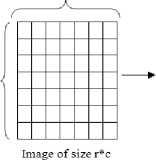
References New Mean-Variance Gamma Method for Automatic Gamma Correction
- 'Image Quality Enhancement Using Pixel-Wise Gamma Correction via SVM Classifier', IJE Transactions B: Applications, Vol. 24, (4), December 2011.
- Tsai, C.M.: 'Adaptive Local Power-Law Transformation for Color Image Enhancement', Applied Mathematics & Information Sciences, 7, (5), 2019-2026 (2013).
- Patel, O., Yogendra P. S., et al.: 'A comparative study of histogram equalization based image enhancement techniques for brightness preservation and contrast enhancement', Signal & Image Processing : An International Journal (SIPIJ), Vol.4, (5), October 2013.
- Nungsanginla, L., Mukesh, K., and Rohini, S.: 'Contrast Enhancement Techniques using Histogram Equalization: A Survey', International Journal of Current Engineering and Technology, 2014, Vol.4, (3).
- Hany, F.: ' Blind Inverse Gamma Correction', IEEE Transactions On Image Processing, Vol. 10, NO. 10, October 2001.
- Yihua, S., Jinfeng, Y., and Renbiao, W.: 'Reducing Illumination Based on Nonlinear Gamma Correction', IEEE. Int. Conf. on Imag. Proce., San Antonio, pp. 529-532.
- Asadi Amiri, S., Hassampour, H.: 'A Preprocessing Approach For Image Analysis Using Gamma Correction', International Journal of Computer Applications (0975 – 8887) Volume 38– No.12, January 2012.
- Shi, J., Cai, Y.: 'A novel image enhancement method using local gamma correction with three-level thresholding', Proc. IEEE Joint. Int. Conf. Information Technology and Artificial Intelligence, vol. 1, Chongqing, China, pp. 374–378, Aug. 2011.
- Gagandeep, S., Sarbjeet, S.: 'An Enhancement of Images Using Recursive Adaptive Gamma Correction', Inter. Jour. of Comp. Scien. and Infor. Tech. (IJCSIT), Vol. 6 (4) , 2015, 3904-3909.
- Yonghun, S., Soowoong, J., Sangkeun, L.: 'Efficient naturalness restoration for nonuniform illumination images', IET Image Process, 2015, Vol. 9, (8), pp. 662 – 671.
- Amandeep, K.: 'Image Enhancement Using Recursive Adaptive Gamma Correction', Inter. Jour. of Innov. in Engin. and Techn. (IJIET), 2014, Vol. 4, (3).
- Parambir, S., Banga, V.K.: 'Dynamic Non-Linear Enhancement using Gamma Correction and Dynamic Restoration', International Journal of Computer Applications, February 2014, Vol. 87, No.12.
- Varghese, A.K, Nisha, J.S.: 'A Novel Approach for Image Enhancement Preserving Brightness Level using Adaptive Gamma Correction', Intern. Jour. of Engin. Resea. & Tech. (IJERT) ISSN: 2278-0181, Vol. 4 Issue 07, July-2015.
- Tan, X., Triggs, B.: 'Enhanced Local Texture Feature Sets for Face Recognition under Difficult Lighting Conditions', IEEE Transactions on Image Processing, Vol.19, 6, pp.1635 - 1650.
- Al-Ameen, Z., Sulong, G., Rehman, A., et al.: 'An innovative technique for contrast enhancement of computed tomography images using normalized gamma-corrected contrast-limited adaptive histogram equalization', Journal on Advances in Signal Processing, 2015, DOI: 10.1186/s13634-015-0214-1.
- Jung, J., Ho, Y.: 'Low-bit depth-high-dynamic range image generation by blending differently exposed images', IET Image Process., 2013, Vol. 7, Iss. 6, pp. 606–615.
- Fedias, M., Saigaa, D.: 'A new approach based on mean and standard deviation for authentication system of face', 2010, International Review on Computers and Software, Vol. 5, (3).
- Gonzalez, R.C., Woods, R.E.: 'Digital Image Processing' (Prentice Hall, 2008, 3rd Ed.).
- Chiu, Y.S., Cheng, F.C., and Huang, S.C.: 'Efficient Contrast Enhancement Using Adaptive Gamma Correction and Cumulative Intensity Distribution', Proc. of IEEE Int. Conf. on Syst. Manag. and Cybernetics, Anchorage, AK. 2011, Oct, p. 2946–50.
- Huang, S.C., Cheng, F.C., and Chiu, Y.S.: 'Efficient Contrast Enhancement Using Adaptive Gamma Correction With Weighting Distribution', IEEE Transactions On Image Processing, Vol. 22, No. 3, March 2013.
- Garg, G., Sharma, P.: 'An Analysis of Contrast Enhancement using Activation Functions', International Journal o f Hybrid Information Technology, 2014, Vol.7, No.5, pp.2.
- Wang, Z., Bovik, A.C., et al.: 'Image Quality Assessment: From Error Measurement to Structural Similarity', IEEE Transactions On Image Processing, Vol. 13, No. 1, January 2004.
- http://vision.ucsd.edu/~leekc/ExtYaleDatabase/ExtYaleB.html. Time accessed: September 2016.
- Lee, K.C., Ho J., Kriegman, D.: 'Acquiring Linear Subspaces for Face Recognition under Variable Lighting', IEEE Trans. Pattern Anal. Mach. Intelligence, 2005, vol.27, No 5, pp. 684-698.
- http://www.cs.dartmouth.edu/farid/#jumpTo. Time accessed: September 2016
- Tarun, A. Arora, Gurpadam, B. Singh, Mandeep C. Kaur: 'Evaluation of a New Integrated Fog Removal Algorithm IDCP with Airlight', I.J. Image, Graphics and Signal Processing, 2014, 8, 12-18, DOI: 10.5815/ ijigsp.2014.08.02
