No-Reference JPEG image quality assessment based on Visual sensitivity

Published Online February 2011 in MECS

Image quality evaluation plays an important role in processing image. With the extensive application of image, developing image quality metric without reference image has received widespread attention especially when it is difficult to obtain reference image. Thanks to image serving people, image quality assessment is more and more dependent on the characteristics of human visual system (HVS). Considerable volume of research has demonstrated that image quality evaluation methods considering human visual characteristics is better than others not considering these characteristics [1]. Therefore, it is imperative to develop the no-reference image quality metric based on human visual factors.

In the last few decades, extensive valuable research has been carried out in developing this topic. Gastaldo et al. proposed a circular back propagation (CBP)-based image quality evaluation method [1], Venkatesh Babu et al. proposed a no-reference image quality index using growing and pruning radial basis function (GAP-RBF) [2] and Suresh et al. proposed a no-reference metric based on extreme learning machine classifier [3].

JPEG is one of the most popular and widely used image formats in internet and digital cameras. In this paper, for JPEG images, the extracted visual sensitivity approach is used to assessment the visual quality of images without any reference. The key human visual sensitivity factors were used as input vectors of network. Image quality estimation includes computation of functional relationship between HVS features and subjective test scores. Here, the functional relationship is approximated using support vector regression neural network. The experimental results show that the proposed no-reference image quality metric has a good consistency with mean opinion score (MOS), really embodying the role of HVS features in image quality measurement.

Zhang You-Sai and Chen Zhong-Jun done the research work together in Jiang Su University of science and technology, and were grateful for LIVE database supported by Prof. H.R. Sheikh, etc.

A key distortion of JPEG images is horizontal and vertical blocking artifact generated by DCT-based transform coding for per 8×8 image block. In order to measure this kind of distortion accurately, several important human visual sensitivity factors such as edge amplitude and length, background activity and luminance [4] are taken into consideration. Given a gray scale image of size M x N . The intensity of the image at any pixel location ( i , j ) is given by I ( i , j ) . The algorithm is explained for extracting human visual features along horizontal direction.

'

Here, Pv = median (Pv), Pv = Pv (8 n),

P v ’( n ) = P v (8 n ) , D h

M P v - P ) •

to Edge amplitude and length: Edge amplitude quantifies the strength of edge along the borders of 8×8 blocks; Edge length quantifies the length of continuous block edges. They are obtained by horizontal orthogonal sobel filter operator.

E

\ I * P\, \ I * P \ < T e

0, others

P is the sobel horizontal filter, E is edge information. Threshold T e should be below 40, if choosing a lower threshold might result in missing the real blocky edges resulting from compression.

to Background activity: Background activity is denoted by the amount of high frequency texture content around the block edges. It is extracted by following method:

M h

1, 0,

I ¹ * F ah \ < ^T a others

Here, _{F ah} is high-pass filtering, M _h is background activity. The value of threshold T a in our experiments is 0.3, the effect of blockiness is masked by the activity if T a is more than 0.3.

Here, P_v is row vector of horizontal sensitivity features, median ( • ) is a five tap median filter, P _v (8 n ) denotes only extracting values of the borders of 8×8 blocks.

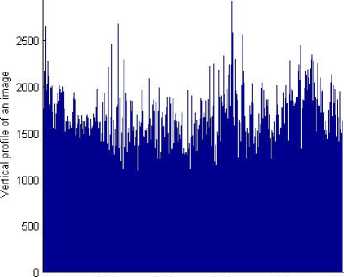
In order to explain this process clearly, the vertical profile and median filtered profile of single image in horizontal direction is shown in Fig.1 and Fig.2, it is explicit that there is sharp rise between both neighboring locations because of block compression, which is in line with Reference [1]. Generally speaking, the more the compression ratio, the greater the rise value and the difference of both reflect human being’s different sensitivity for different area in an image. The sensitivity difference is shown in Fig.3.

Similar steps are used to obtain the sensitivity difference along vertical direction ( DV ). The final sensitivity difference ( DF ) is got by combining the horizontal and vertical sensitivity difference (Dp = [D„, D ]). The HVS feature vector X is able F HV to be obtained by quantizing DF into 14 intervals. The 14 intervals are divided as following way: [min,-1) , [-1,-0.6) , [-0.6,-0.3) , [-0.3,-0.1) , [-0.1-0.05), [-0.05,-0.01), [-0.01,0), [0,0.05], (0.05,0.1] , (0.1,0.3] , (0.3,0.6] , (0.3,1.5] , (1.5,2.5], (2.5, max].

to Background luminance: Background luminance measures the amount of brightness around the block edges. It is obtained by following way:

The extracted HVS feature from 233 JPEG images is showed in Fig.4. Here, x axis, y axis and z axis respectively denote dimension per image, the number of sample images and corresponding HVS feature. It can be observed from Fig.1 that most of HVS features fall in the range of (-1, 0.3) and evenly distributed feature could ensure difference of different images.

Wi (i, j) =

I * fl p 128

1

0 < I(i, j) < 128

others

Here, fl_p is low-pass filter, W_l is background luminance.

to Obtain the combined sensitivity difference along the horizontal direction ( D_H ):

0        100       200 .Ш 400      500       600

Horizontal pixel number of an image

Fig.1 The vertical profile of an image

P v ( i ) = f Е_л ( i , j ) x M_h ( i , j ) x W ( i , j )   (4)

j = 1

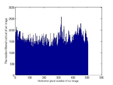
Fig.2 The median filtered profile of an image

features and mean opinion score. The HVSOS index considers human visual sensitivity factors as a criterion to evaluate the image quality, so the image visual quality is emphasized and then the process of image quality assessment is to some extent simplified.

A. The basic principles of SVR-NN

The basic idea of SVR-NN algorithm is that architecture of SVR-NN is initialized by SVR and then corresponding parameters of network is updated using neural network. In this paper, we select 8 — SVR for initializing architecture of SVR-NN because of its better sparsity performance and Gaussian function as kernel function of SVR-NN because of its better performance of fitting. Therefore, the architecture of SVR-NN can be written as [5]:

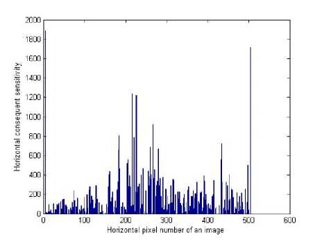
Fig.3 Horizontal consequent sensitivity difference

s

f (x)=E (a a*)exp i=1

— x'i 1 , (5)

к 2Y )

Here, a i is vector solution, a i is dual vector solution, 5 denotes the number of support vector, v and / are center vector and width of the hidden node.

B. HVSOS metric approach model

Mentioned above, HVSOS model applied in image quality is constructed as Fig.2:

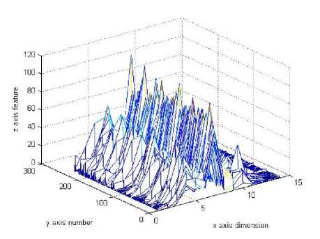
Fig.4 Illumination of HVS features

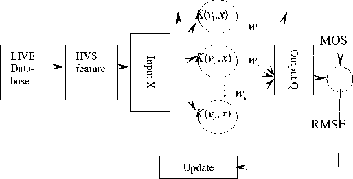
Fig.2 the HVSOS metric model of image quality

From Fig2, it is shown that the architecture of HVSOS index is regarded as a two-layer neural linear network and in order to beat the target of MOS convergence, neural network updates weight vector, center vector and width of the hidden node of SVR-NN based on the convergence of RMSE.

Because of the goal of image quality assessment for people, the performance of measurement approach considering human visual sensitivity is highly better than those without considering them. Therefore, the human visual sensitivity objective score (HVSOS) is presented to assess image quality. The support vector regression neural network (SVR-NN) is utilized to approximate the functional relationship between human visual sensitivity

ˆ

Q HVSOS

s

E w‘ exp

i = 1

(

^^^^^^^B

к

]2/    )

+ b , (6)

Eq. (6) shows the output result of HVSOS assessment metric. Here, x = [ x 1 , x 2 ,..., x q "T is input sample matrix extracted in section II, 5 denotes the number of support vector, w ' = ( a i — a i ) ^ 0 is weights needed

updating, V and у are center vector and width of the hidden node needed updating, b is bias of network.

To obtain better assessment accuracy, neural network algorithm based on gradient-decent method is used to update SVR-NN network. The lost function for HVSOS is defined here [6]:

E R = л ^(t) а  г e x t ) ) ) , e ( t ) = y_ - y , ⁽ t ) , (7)

£ 2 I   (xt)JJ

Here, t is the epoch number; is the layer number, y ⁾ ( t ) is assessment value. Update the weight vector, center vector and width of the hidden node according to [7]:

a e R S w ', =--— = 9 w ' ,	e, ( t )	a e ,. ( t )
	e 2 ( t ) 1 + —--	d w '

^ ( t )

e (t)

The             in Eq. (8), (9), (10), which resulted

1+eYtLM(. t)

from lost functions such as Eq. (7) has a great impact on the approximation between objective assessment results and MOS especially when there are outliers exist. If

e (t)

1 + e Y t! ц ⁽ t )

weaken too quick, there is not

enough time for most of training data to converge and then evaluation results of HVSOS index are mostly smaller than actual values, that is to say, under fitting occurs; if this decay is too slow, there is too a long time for training data to converge in time, and then assessment results are greater than actual results. Ultimately, the outliers are mistaken as normal training data. That is to say, the over fitting happens.

e j ( t )

1 + e-M Ц⁽ t )

■ exp<

II x - v ||2 2y2

Therefore, the suitable decay method is that u ( t ) = A / 1 is selected, and then the better generalization performance is achieved, especially when A is a constant [6].

S v .,, =

e j ( t ) e ² ( t )

1 + ——

H ⁽ t )

ae,(t) ■---------------------- av,(t)

= w', ■

X- — V- .

i i ,

Г , ²

■ exp<

II x - v, II2 2y J2

e (t)

1 + e^-M⁽ t )

Here, X i is i th dimension of X , i = 1,2,..., q .

e ,. ( t )      a e ,. ( t )

--------------7---

, e ( t ) dy , 1 + ——

Д ( t )

In our simulations, we have used the LIVE image quality assessment database I [8] which is constituted of 29 JPEG original images and 204 JPEG images with different compression rates from original images. The 233 images are divided into two disjoint sets for training and testing. The corresponding MOS need be transformed to 1-10 range. In order to validate the effect of evaluation of proposed HVSOS, Wang’s NR [9], ELM [3] and SSIM index [10] are compared to proposed HVSOS algorithm.

After training phase, the parameters are set as follows:

8 =1.25 , C =31 , y =27 , n =0.1800 , a =0.0200, the number of iteration is 300. The error RMSE convergence curve is shown in Fig.5.

, II x - v , II 2	II X - V , II	e ( t )
1     y3	2 y 2	1 + eYt )

^ ( t )

w,(k+1) = w(k- + n-8w',+ a\w(k- - w‘(k-1)), (11) v<--" = v(‘> + n-Sv.,,+ «-(v!, - v<*-") ■    (12)

y .‘ • ^1I = y , k ¹ + n - Sy , + a- ( y (k ¹ - y , k ^-") ,     (13)

Here, k is the number of iteration n is the learning rate, a is momentum coefficient.

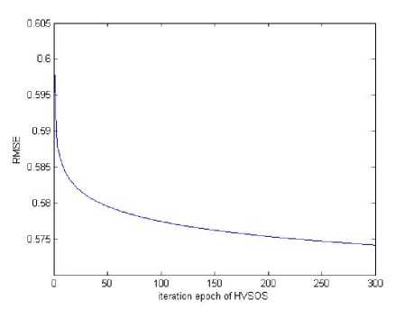
Fig.5 Error convergence curve of HVSOS

• A.    Visual analysis of HVSOS

In our experiments, the LIVE image database is divided into train set and test set. The PSNR and HVSOS are respectively used to predict the train and test sets. Fig.6 and Fig.7 show comparison measurement results for train sets, Fig.8 and Fig.9 for test sets.

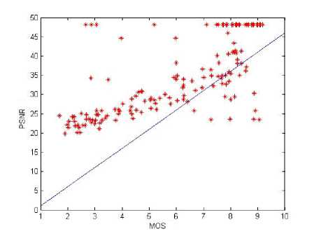
Fig.6 PSNR quality assessment of training sets

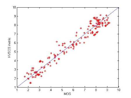
Fig.7 HVSOS quality assessment of training sets

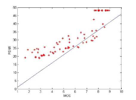
Fig.8 PSNR quality assessment of testing sets

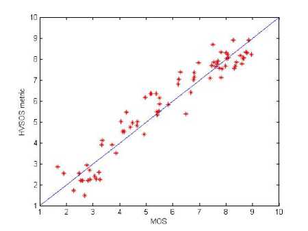
Fig.9 HVSOS quality assessment of testing sets

As can been seen from Fig.6 to Fig.9, whether is train sets or test sets, the evaluation results of HVSOS index are all able to precisely vary with diversification of MOS values, more evenly distributing around the ideal straight line and then there are few outliers interfering with experimental results.

In order to vividly explain this phenomenon, here show four group pictures, such as Fig.10 (a) (b), Fig.11 (a) (b), Fig.12 (a) (b), Fig.13 (a) (b), each of which is composed of both same pictures except the blocking effect. These pictures reveal human visual sensitivity effect in different aspects. There is better visual effect in Fig.10 (a) and Fig.11 (a) than in Fig.10 (b) and Fig.11 (b), because of the (b) pictures’ bad blocking in them; while the both group of Fig.12 and Fig.13 owe the same high visual quality and little visual difference between (a) and (b) of each group.

(a)

(b)

Fig.10 LIVE: churchandcapitol

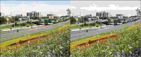
(a)                                   (b)

Fig.11 LIVE: flowersonih35

(a)

(b)

Fig.12 LIVE: woman hat

(a)

(b)

Fig.13 LIVE: cemetery

The table 1 shows each evaluation result that is predicted in HVSOS and PSNR two metrics.

TABLE 1

The comparison of various pictures between HVSOS and PSNR

LIVE Image database		Index
		HVSOS	PSNR	MOS
churchand-capitol	(a)	7.0136	29.8147	6.2800
	(b)	2.5153	26.5907	2.6809
flowersonih35	(a)	4.6156	22.2849	4.0492
	(b)	1.5945	20.2892	1.6803
woman hat	(a)	8.4810	48.1308	8.9675
	(b)	7.9951	38.0535	8.2422
cemetery	(a)	7.7467	48.1308	7.8412
	(b)	7.7244	32.2077	7.3663

Seen from table 1, it is obvious and precise that the HVSOS index gave right difference for big difference between Fig.10 (a) and Fig.10 (b), so is it for Fig.11 (a) and Fig.11 (b); while the PSNR index assesses the very similar evaluation results, which is not consistent with the corresponding MOS values. For the Fig.12 (a) and

Fig.12 (b), they have close visual quality. This is highly consistent with HVSOS index’s evaluation result and MOS value, which is contrary to PSNR giving assessment results for Fig.13 (a) and Fig.13 (b).

• B.    The comparison between HVSOS approach and other popular metrics

TABLE 2

Comparison of various metrics

	Training sets		Testing sets
Metrics	RMS E	R-squa re	RMS E	R-squa re	Ty pe
Wang’s NR	4.690 0	-2.3930	5.090 0	-2.5170	NR
ELM	0.690 0	0.9010	0.700 0	0.9230	NR
SSIM	0.630 0	0.9408	0.650 0	0.9431	FR
HVSOS	0.577 6	0.9378	0.613 1	0.9201	NR

From TABLE 2, obviously, the RMSE value of HVSOS model is much less than that of other three algorithms and the R-square value of HVSOS are much more excellent than that of Wang’s NR and SSIM algorithms. Therefore, we could conclude that the proposed HVSOS quality model owns better generalization performance and its measurement result has a higher consistency with HVS features.

In this paper, a novel HVSOS metric approach is presented to assessment the visual quality of JPEG-coded images considering various HVS features. The functional relationship between the extracted HVS features and MOS is modeled by SVR-NN. The network can be updated easily and the performance of the proposed metric is better than others. This metric can be easily extended to measure the quality of videos which also use similar block DCT-based compression.

The authors would like to express their thanks to Prof. H.R. Sheikh and Prof. Bovid for providing the JPEG image quality assessment database to validate our metric.

• [1]    P.Gastaldo , R.Zunino, “No-Reference Quality Assessment of JPEG Images by Using CBP Neural Networks, ” IEEE Internationa1 Symposium on Circuits and Systems , pp.772-775, May2004.

• [2]    R. Venkatesh Babu, S. Suresh, Andrew Perkis , “No-reference JPEG-image quality assessment using GAP-RBF,” Signal Processing of ScienceDirect , A87, 2007, pp.1493-1593.

• [3]    S. Suresh, R. Venkatesh Babu, “H.J. Kim. No-reference image quality assessment using modified extreme learning machine classifier,” A pplied Soft Computing of ScienceDirect , pp.541–552, September2009,

• [4]    S.A. Karunasekera, N.G. Kingsbury, A distortion measure for blocking artifacts in images based on human visual sensitivity, IEEE Transactions on Image Processing , 4 ^th ed., pp.713-724, June1995.

• [5]    C-C Chuang, S-F Su, “Robust Support Vector Regression Networks for Function Approximation with Outliers,” IEEE Trans on Neural Networks , 13 ^th ed., pp.1322-1330, June2002.

• [6]    C-C Chuang, S-F Su, C-C Hsiao, “The annealing robust backprogagation (ARBP) learning algorithms,” IEEE Trans on Neural Networks , 11 ^th ed., pp.1067-1077, May2000.

• [7]    Li Jun, Liu Junhua, “Identification of dynamic systems using support vector regression neural networks,” Journal of Southeast University (English Edition) , pp.228-233, June 2006,.

• [8]    H.R. Sheikh, Z. Wang, L. Cormack, A.C. Bovik, “Live image quality assessment database”, website: http://live.ece.utexas.edu/research/quality .

• [9]    P.Gastaldo , R.Zunino , “No-Reference Quality Assessment of JPEG Images by Using CB PNeura1 Networks,” IEEE Internationa1 Symposium on Circuits and Systems , pp.772-775, May2004.

• [10]    Z. Wang, A.C. Bovik, H.R. Sheikh, E.P. Simoncelli, “Image quality assessment: from error visibility to structural similarity,” IEEE Trans. Image Process . 3 ^rd ed., pp.600-612, April2004.

Prof. Zhang You-Sai, who was born in 1959, Zhenjiang city, Jiangsu Province, researches on image processing and 3D visualization;

Chen Zhong-Jun, who was born in 1983, He Nan province, researches on image and video processing.

Communication author:

Zhang You-Sai, Jiang Su University of science and technology, 2# Meng Xi Road, Zhen Jiang city of Jiang Su province in China.

Mobile Phone: 13862442688