Noise Removal From Microarray Images Using Maximum a Posteriori Based Bivariate Estimator

Published Online January 2013 in MECS

The arrival of microarray imaging technology has lead to enormous progress in the life sciences by allowing scientists to analyze the expression levels of thousands of genes at a time. It is a powerful tool for discovering various types of diseases and for diagnosing the type of disease based upon gene expression measurements. But the noise introduced in microarray images gives rise to a challenge for engineers to interpret the meaning of the immense amount of biological information formatted in numerical matrices from the expression levels of thousands of genes, possibly all genes in an organism.

The two-channel complementary DNA (cDNA) microarray is designed to measure the activity of a set of genes under two conditions, namely, treatment and control [20]. A typical cDNA microarray experiment consists of the following major steps. Messenger RNA from control and treatment samples are converted into cDNA, labeled with fluorescent dyes (green Cy3 dye for control, red Cy5 dye for treatment) and mixed together. The mixture is then washed over a slide spotted with probes, which are DNA sequences from known genes. During this stage, competitive hybridization occurs, which is the pairing of the fluorescent cDNA to the spotted probes. Next, the slide is scanned to produce two 16-bit images, one for the green channel and another for the red. Each spot on the images consists of a number of pixels, wherein the brightness of each pixel reflects the amount of Cy3 or Cy5 at the spatial location corresponding to that pixel. Thus, one can identify the genes that are differentially expressed between the two samples by comparing the pixel intensities of each spot in the red and green channel images.

This paper introduces a technique for removing noise from microarray images based on Complex Wavelet Transforms. There are two major approaches of statistical wavelet-based denoising algorithms. In the first approach, the wavelet coefficients are modified using certain threshold parameters and shrinkage functions. The second and better approach is to formulate the denoising algorithm as an estimation technique for the noise-free wavelet coefficients of images by minimizing a Bayesian risk, typically under the Minimum Mean Squared Error (MMSE) or Maximum A Posteriori (MAP) criterion . Denoising algorithms that assume the wavelet coefficients of the entire subband are independent and identically distributed (i.i.d.), are called subband-adaptive.

• II.    RELATED WORK

Studies show that microarray images are corrupted by several types of noise that result from the imaging system. Some examples of these noises include electronic noise, photon noise, dark current noise, and quantization noise [9], [21]. Noise may also be introduced from other sources such as nonspecific hybridization to the probes on the microarray surface and dust on the glass slide [22]. Statistical distributions such as the Gaussian [9], Poisson [1] and Exponential distributions [5] have been used to describe the noise characteristics of microarray images considering additive or multiplicative noise model [2]. It is to be noted that many non-additive and non-Gaussian noise models for images can be mathematically remodeled as the additive Gaussian noise. Since the underlying processes that generate noise in the red and green channel images of cDNA microarrays are similar, it is expected that the noise are correlated between the two channels. The reduction of such correlated Gaussian noise is an important problem for processing of microarray images. Reduction of noise from microarray images can be performed in the pixel-domain [9], or in a transform domain [18].

Although the pixel-based methods are simpler to implement in general, methods developed using an appropriate transform domain are more efficient in reducing noise. Among the various transforms, the Discrete Wavelet Transform (DWT) has shown a significant success in image de-noising due to its space-frequency localization and high energy compaction properties, and flexibility of choosing a suitable basis function [10]. Further, the DWT being a multi-resolution analysis allows one to efficiently process an image at more than one resolution. For this reason, the DWT is gaining attention among researchers for developing new techniques to conduct several tasks in the microarray experiments such as gridding, spot recognition and analysis of differential gene expression [17]. A wavelet-based noise reduction algorithm may be embedded into the routines of such wavelet-based techniques for analyzing gene expression data so that the entire process of image processing and data analysis becomes faster, automated, and efficient. The Complex Wavelet Transform (CWT) is preferred to the discrete wavelet transform for de-noising of microarray images due to its improved directional selectivity for better representation of the circular edges of spots and near shift-invariance property.

The better approach is to formulate the denoising algorithm as an estimation technique for the noise-free wavelet coefficients of images by minimizing a Bayesian risk, typically under the Minimum Mean Squared Error (MMSE) [15] or Maximum A Posteriori (MAP) criterion [11]. Denoising algorithms that assume the wavelet coefficients of the entire subband are independent and identically distributed (i.i.d.), are called subband-adaptive. It is well known that the wavelet coefficients have strong intrasubband and weak interscale dependencies. Hence, locally-adaptive methods that estimate a wavelet coefficient from its local neighboring region provide a better denoising performance as compared to the subband-adaptive ones. A few methods have considered both the intrasubband and interlevel dependencies while denoising an image [12]. These methods provide slightly better denoising performance than those that use only intrasubband dependency, but at the expense of increased computational complexity. In this paper, two bivariate estimators namely Maximum A Posteriori (MAP) and Linear Minimum Mean Squared Error (LMMSE) are presented for the CWT-based denoising of microarray images.

• III.    DENOISING USING COMPLEX WAVELET TRANSFORM

The Complex Wavelet Transform (CWT) differs from the DWT in having complex-valued scaling and wavelet functions, viz., ɸ 1 + j ɸ 2 and ψ 1 + jψ 2 , respectively, and form Hilbert pairs [13], [14]. Various methods have been proposed for obtaining CWT coefficients [8], however, due to the simplicity of implementation and lower redundancy, the dual-tree CWT (DT-CWT) that has been proposed by Kingsbury [8] and later generalized by Se-lesnick [13], is becoming popular. The DT-CWT consists of two trees of DWT in parallel and provides four pairs of sub-bands (Figure.1). The implementation of DT-CWT requires that the functions ɸ 1 and ψ 1 operate on the odd numbered data samples, and ɸ 2 and ψ 2 operate on the even numbered data samples.

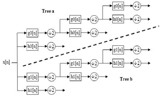
Figure 1: DT-CWT sub-band decomposition

Thus, in general, processing of the magnitude components of an image is more efficient than that of the phase components. The choice of scaling and wavelet functions of DT-CWT is such that this transform can capture six directional features, namely, 15, 45 and 75 and -15,-45,and -75 degrees of an image. Hence, the CWT provides a better directional selectivity as compared to the DWT that has only three angle-selective sub-bands. In order to improve the shift-invariance property, the DT-CWT avoids down-sampling operation in the first-level decomposition. Hence, the CWT has much lower shift sensitivity than the DWT.

• A.    Estimation of CWT Coefficients

Let fr(i,j) and fg(i,j) be pixels of the red and green channel images, respectively, at the spatial location. Assume that these pixels are corrupted by additive noise. Then, the noisy pixels are given as in (1), gr(i,j)= fr(i,j) + εr(i,j)

g g (i,j)= f g (i,j) + ε g (i,j) (1)

Where εr(i,j) and εg(i,j) are the noise samples at reference location. It is assumed that noise-samples of the red and green channel images are correlated and distributed as i.i.d. zero mean bivariate Gaussian having equal variance σε2 and correlation coefficient ρε. The standard deviation σε indicates the strength of noise and ρε measures the amount of linear dependency of noise between channels.

• B.    Denoising Algorithm

De-noising algorithm (Figure.2) consists of the following steps:-

• 1)    Add Gaussian noise of different strengths and compute the Complex Wavelet Transform of the noisy image.

• 2)    Modify the noisy wavelet coefficients according to LMMSE and MAP estimators,that take into account the inter-channel dependency of the magnitude components of CWT coefficients of the image.

• 3)    Compute the Inverse Complex Wavelet Transform using the modified coefficients for getting the denoised image.

• 4)    Perform Gridding and Segmentation of de-noised image in order to estimate the Log Intensity Ratio.

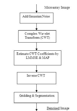
Figure 2: Steps for denoising microarray images

The wavelet coefficients in the lower level subbands are dominated by noise unlike that in the higher levels. As a consequence, overall denoising performance is highly dependent upon the efficiency of noise removal from the subbands at the lower levels. In other words, it is more important to choose a joint probanility density function (pdf) that provides a better fit to the magnitude components of the subbands in a lower level to achieve a satisfactory denoising performance. Hence, for the purpose of denoising, the bivariate Gaussian pdf is an appropriate choice. In addition, an attractive feature of bivariate Gaussian pdf is that it is mathematically tractable for developing an estimator. So the bivariate LMMSE and MAP estimators are derived using this pdf as a joint prior function [16].

• C.    Bivariate LMMSE Estimator

Let x = [x r ,x g ]^T, y = [y r ,y g ]^T and v=[v r ,v g ]^T be the samples of the random vectors X,Y and V representing magnitude components of the noise-free coefficients, noisy coefficients and noise coefficients respectively. The

LMMSE estimator for x given the corrupted observation y is a linear function of y that can be written in (2), x = Mx + exy ZV(y - My )                  (2)

Where µ X and µ Y are the mean of the random vectors X and Y, Σ XY is the cross-covariance matrix of X and Y,and Σ Y is the covariance matrix of Y . The matrices may be written as in (3) and (4),

E xy = E{(X - M x )(Y - M y ) T }           (3)

and

E Y = E {( Y - M y )(Y - M y ) T }              (4)

Where E{.} is the mathematical expectation. Since the image and additive noise are independent, μ Y = μ X + μ V and Σ_XY = Σ_X, where μ_V is the mean vector of V, μ_X is the mean vector of X, and Σ_X is the covariance matrix of X .

• D.    Bivariate MAP Estimator

The MAP estimator for x given the corrupted observation y is the mode of the posterior density function ρ X|Y ^(x|y) and is given in (5).

x , ( У ) = argmax( P xY ( x | y))

(or)

x ( y ) = argmax[ln( p V ( y - x ) + In p _X ( x )]            ⁽⁵⁾

x

Where ρ X (.) is the bivariate Gaussian pdf and ρ V (.) is the bivariate Rayleigh pdf. Then the bivariate MAP estimator for red and green channel images is given in (6).

л               i /7          \              r^г

1        I 2.2              2        22

x r = max(--------- — I I 2 ff _r + Q _v l y _r + M r ^ v - ^ v ( У г - M r )

2(^2 + aV)

+ 4 a r4 a V + 4 a r a 4 1 ,0)

,        1        I 2.2                2        2               2        4   2        24

x g = max(-------— H2 » g + a ) y g + M g a - ^ a ( У д - M g ) + 4 a g a + 4 a g a v

2( a 2 + a V ) V

• E.    Log Intensity Ratio(R) Estimation

The purpose of microarray image denoising is to improve the extraction of information regarding gene expression levels instead of visual enhancement as in traditional image denoising. Therefore, a successful microarray denoising algorithm is one that reduces noise with minimal loss of information for downstream statistical analysis. In cDNA microarray experiments, information regarding gene expression is commonly expressed in terms of the log-intensity ratio(R) that is given in (7),

R = log 2

11n E S .1n E S

V      S g

^- b r

—

b g

У

Where Sr and Sg denote the pixels of red and green channel images respectively and n is the number of pixels in the region of interest(ROI) and br and bg are the median of the pixels of local background corresponding to the ROI of two channels.

To calculate R, the first step is to identify target areas in the red and green channel images. In general, the target area is a square or rectangular region on an image enclosing one spot. These regions are identified by placing a grid over the entire image. The next step, known as segmentation, consists of identifying the pixels that belong to the ROI and background in a target area. There exist several segmentation methods, each having certain advantages and drawbacks. Some of these methods have been compared in [22] and [19]. In this paper, an adaptive segmentation technique is implemented that is a hybrid of the fixed circle-based [3] and histogram-based [7] segmentation methods, in order to benefit from the advantages of both these methods. Segmentation is performed separately for the red and green channel images.

The hybrid segmentation method has the following two notable features that make it superior to the traditional fixed circle and histogram-based segmentation methods. First, the ROI selected by this method does not assume any perfectly circular shape at the center of target area as in the case of fixed circle-based method. Thus, the hybrid method provides a better separation of foreground when the spots have varying radii, irregular shapes, or spatial offsets from the center of the target area. Secondly, in selecting the pixels for a spot and its corresponding background the hybrid segmentation method considers the spatial contexts that are ignored in the histogram-based method.

• IV.    IMPLEMENTATION DETAILS

  The experiments are conducted on a set of microarray images that have been downloaded from the website of the Stanford MicroArray Database[23] and [24]. In order to conduct the experiments original noise-free images are necessary. Since perfectly noise-free images are not available in practice, noise-free images those that appear to be corrupted with very little noise are chosen.The images that have been used in the experiments are of size1000 x 1000 in 16-bit tagged image file format (.TIFF). The algorithm is implemented in MATLAB.

• A.    Algorithm

Input: Noisy microarray image

Output: De-noised image begin

Symmetric extension of noisy image by calling symextend function do

Apply DT-CWT by calling cplxdual2D function until level<=4

Modify CWT coefficients by calling lmm-se_estimator or map function do

Apply inverse DT-CWT by calling icplxdual2D function until level<=4 end

• B.    User Defined Functions

The functions implemented are discussed below in detail.

• •    symextend(x,2^N(J-1)): This function performs the

symmetric extension of the pixels in the noisy image by taking the noisy pixel values ( x ) and the number of levels ( J ) as inputs.

• •    cplxdual2D(x, J, af, sf): This function calculates the DT-CWT coefficients by taking the noisy image ( x ), number of levels ( J ), analysis ( af ) and synthesis ( sf ) filter results for trees as arguments.

• •    normcoef(W,J,nor): This function calculates the normalized coefficient values by taking the noisy CWT coefficients ( W ) and number of DT-CWT stages ( J ) as inputs.

• •    expand(Y_parent_real): This function expands the

real coefficient values.

• •    expand(Yparent imag): This function expands the imaginary coefficient values.

• •    lmmse_estimator(Y_coef,Y_parent): This function

estimates the LMMSE estimator values by taking the noisy CWT coefficients ( Y_coef ) and parent coefficients ( Y_parent ) as inputs.

• •    map(Y_coef,sigmar,sigmag,m1,m2): This function calculates the MAP estimator values by taking the noisy CWT coefficients ( Y_coef ), standard deviation ( sigmar,sigmag ) and mean ( m1,m2 ) of red and green channel images as arguments.

• •    bishrink(Y_coef,Y_parent,T): This function modi

fies the noisy CWT coefficients by taking the estimated CWT values ( Y_coef ), parent coefficient ( Y_parent ) values and threshold ( T ) values as inputs.

• •    icplxdual2D(W, J, Fsf, sf): This function performs inverse DT-CWT operation by taking estimated coefficient values ( W ), number of decomposition levels ( J ) and synthesis filter ( Fsf, sf ) results as inputs.

• C.    Assessment Measures

The de-noising performance of the algorithm is quantified in decibels (dB) using the peak signal-to-noise ratio (PSNR) which is given in (8).

( 65535² )

65535 I                      (8)

MSE ( f ') )

Where MSE(f’) is the mean squared error of the denoised image f’. This measure is inversely proportional to the residual error in an image.

Signal-to-noise ratio (often abbreviated SNR or S/N) is a measure used in science and engineering to quantify how much a signal has been corrupted by noise. It is defined as the ratio of signal power to the noise power corrupting the signal. A ratio higher than 1:1 indicates more signal than noise.

I(r,c)2

SNR ^----

MSE

Where MSE is the Mean Squared Error which is the difference between the original image and the denoised image and I means original image (without noise), r means row, and c means column of the microarray image.

Image fidelity (IFy) refers to the ability of a process to render an image accurately, without any visible distortion or information loss. Image fidelity is measured in physical characteristics (luminance, dynamic range, distortion, resolution, and noise) and with psychophysical techniques, including receiver operator characteristics analysis with clinical images and testing with contrast-detail patterns to determine threshold contrast.

IFy = 1 -

SNR

Where SNR is the Signal to Noise Ratio.

Image quality is a characteristic of an image that measures the perceived image degradation (typically, compared to an ideal or perfect image). Imaging systems may introduce some amounts of distortion or artifacts in the signal, so the Correlation Quality (CQy) assessment is an important problem.

CQy

E I (r, c )* Id (r, c)

EI ( r, c )

Where for an image of R*C (rows-by-columns) pixels, r means row, c means column, I means original image (without noise), and I d means denoised image.

Image quality loss resulting from artifacts depends on the nature and strength of the artifacts as well as the context or background in which they occur. In order to include the impact of image context in assessing artifact contribution to quality loss, regions must first be classified into general categories that have distinct effects on the subjective impact of the particular artifact. These effects can then be quantified as Structural Content (SCt) which is used to scale the artifact in a perceptually meaningful way.

SCt =

E I ( r , c ) 2

^E I d ^{( r},^{c ) 2}

Where for an image of R*C (rows-by-columns) pixels, r means row, c means column, I means original image (without noise), and I d means denoised image.

• V.    EXPERIMENTAL RESULTS

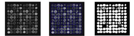
Noisy images are created by adding bivariate Gaussian noise to the noise-free images considering four values of standard deviation, viz., 500, 600, 700,and 800. Figure 3 and Figure 4 shows the denoising results of a microarray image by applying Dual tree Complex Wavelet Transform on both red and green channel images separately. Also, Figure 5 represents the Gridding and Segmentation steps of the denoised images needed for the estimation of log intensity ratio.

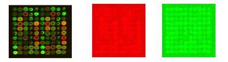
(a)                      (b)                   (c)

Figure 3: (a) Noise free Microarray Image Array 1. (b) Noisy Red Channel Image. (c) Noisy Green Channel Image. Here Noisy images are formed by adding Gaussian noise of standard deviation σ=500

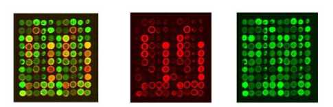
(a)                     (b)                   (c)

Figure 4: Denoised Images obtained by applying Dual Tree Complex Wavelet Transform (a) Denoised Image (b) Red channel Image (c) Green Channel Image

Calculated PSNR values are tabulated in Table 1.Higher PSNR implies a better noise reduction performance. Also, the log-intensity ratio values are estimated from the denoised images. Table 2 tabulates the average PSNR values and Log intensity ratio estimated using both LMMSE and MAP estimator techniques by applying different noise strengths on the microarray images.

(a)                   (b)                    (c)

Figure 5: (a) Denoised Image (b) Gridding (c) Segmentation

Based on the estimated Log intensity ratio (R) values, the expression of genes in the microarray images are measured as follows.

V R=0 means gene is expressed equally in both control and treatment sample.

V R<0 means gene is expressed more in control sample.

V R>0 means gene is expressed more in treatment sample.

Table 1: PSNR values estimated in Db at various Noise Strengths for Microarray Image Array1

Standard Dev-iation(a)	500	600	700	SOO
LMMSE	40.12	39.78	38.52	36.89
MAP	42.47	41.42	39.99	3S.7S

Table 2: Average PSNR values and Log intensity ratio estimation of Stanford Microarray Database Images

Images	PSNR(average in dB)		Log Intensity Ratio(R)
	LMMSE	MAP	LMMSE	MAP
Array 1	3S.S3	40.66	0.09S	0.090
Array?	35.67	37.09	0.126	0.121
АггауЗ	3S.56	39.OS	0.100	0.09S
Array4	41.77	42.64	0.109	0.105

Figure 6 shows the denoising results of another microarray image obtained by applying Dual tree Complex Wavelet Transform on both red and green channel images separately. Figure 7 shows the PSNR values estimated for different noise strengths by both LMMSE and MAP estimator method for two microarray images. It shows that, increase in Noise Strength decreases the PSNR Values. This implies that when more noise is present, performance of LMMSE and MAP decreases. The algorithm gives good results for the Gaussian noise having standard deviation below 750.

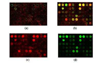
Figure 6: (a) Noisy Image Array2 (b) Denoised image (c) Denoised red channel image (d) Denoised green channel image

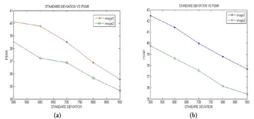
Figure 7: Performance analysis ofproposed method (a) LMMSE method and (b) MAP method.

The other assessment parameters that are used to evaluate the performance of noise reduction of microarray images are Signal to Noise Ratio (SNR), Image Fidelity

(IFy), Correlation Quality (CQy), and Structural Content (SCt). These parameters are estimated for determining the quality of denoised microarray images. Table 3 shows the estimated parameter values for the given denoising algorithm.

The presented denoising method based on DT-CWT is compared with the existing BiShrink Method for calculating CWT coefficients proposed by I.W.Selesnick. Table 4 tabulates the average PSNR values calculated by LMMSE, MAP estimators and BiShrink Method. Also, compared with other de-noising techniques by applying filters like median and wiener at various noise strengths by adding Gaussian noise. Table 5 and Table 6 tabulates the assessment parameters like PSNR, SNR, Image Fidelity (IFy), Correlation Quality (CQy), and Structural Content (SCt) estimated by applying Median filter and Wiener filter on various microarray images. Higher values of SNR show better de-noising performance.

Table 3: Performance Measurements

Images	SNR	IFy		SGI
Ar rayl	3.777	0.749	159.549	0.5413
Array!	3.S54	0.741	158.910	0.5387
Array)	3.659	0.745	157.761	0.5409
Ar ray4	3.SS2	0.75S	160.555	0.5217

Table 4: Performance Comparison

Image	BiShrink	LMMSE	MAP
Array 1	25.66	32.23	33.55
Array!	30.22	35.67	37.09
АггауЗ	32.71	38.56	39.08
Array4	35.07	41.77	42.64
Array5	34.22	40.23	41.55

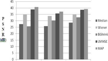
Figure 8 shows the average PSNR values estimated in dB for microarray images by applying Gaussian noise and using techniques like LMMSE, MAP, BiShrink method, Median and Wiener Filters. From the Figure 8, it is understood that the proposed LMMSE and MAP Estimator techniques show better de-noising performance than other methods. Also, Wiener filter results shows better denoising performance than Median filter and BiShrink method.

Table 5: Performance measures of Median filter

Images	PSNR	SNR		CQy
Array 1	27.3776	2.754	0.612	150.456	0.654
Arrav2	25.7SSS	3.176	0.654	148.560	0.588
Array)	28.5677	2 545	0.674	152.226	0.532
Array 4	29.2391	3.987	0.693	155.132	0.515

Table 6: Performance measures of Wiener filter

Images	PSNR	SNR	Ki	СЖ	SQ
Array 1	34.9090	3.467	0.712	155.456	0.529
Array!	33.7123	3.345	0.709	153.560	0.562
Array)	34.9061	3.477	0.741	158.226	0.531
Arrav4	35.2189	3.545	0.791	159.132	0.520

Microarray Images

Figure 8: Comparison of PSNR values of various methods

Hence, the experimental results obtained by conducting the five denoising experiments on the available microarray data set shows that the denoising algorithm using DT-CWT with MAP estimator outperforms the other denoising algorithms.

• VI.    CONCLUSION

The cDNA microarray images are contaminated by different sources of noise that are introduced during various steps of the microarray experiments. The noise must first be reduced from these images for extraction of accurate gene expression measurements. In this paper, two CWT-based denoising methods have been implemented for microarray images using the standard MAP and LMMSE estimation criteria. The main strength of the proposed denoising methods is that unlike existing methods that are capable of processing each image separately, the proposed bivariate estimators incorporate the correlation information of the images as well as noise between the red and green channels. The experimental results show that the MAP estimator technique shows better denoising performance than other existing denoising techniques.