Non Intrusive Eye Blink Detection from Low Resolution Images Using HOG-SVM Classifier

Published Online October 2016 in MECS

The field of Human Computer Interaction (HCI) has seen a lot of changes in the past few years. The traditional user interfaces such as keyboards, mouse, touch screen etc are being replaced by Natural User Interfaces (NUI) that rely on human gestures [1], facial expressions [2], eye movements[3] etc. Among them the interfacing systems that uses eye movements and eye blinks as inputs has a vital role in designing communicative interfaces for people who has limited motor abilities. The diseases like cerebral palsy or Amyotrophic Lateral Sclerosis (ALS) prevents patients from interacting with computers like normal people. In such cases, special communication devices have to be developed that relies on the patient’s eye movements, eye blinks etc.

The aim of this paper is to develop an effective nonintrusive eye blink detection method that can be used in such systems which work under different lighting conditions and use low cost imaging devices which provide low resolution eye images. This paper presents five methods using a combination of features like Fisher Faces, Histogram of Oriented Gradients (HOG), Local Mean Intensity and classifiers like Artificial Neural Networks (ANN) and Support Vector Machines (SVM) as classifiers. The accuracy of each method was compared for different number of training images. The combination of HOG features with SVM turned out to be the most accurate of all methods. The accuracy of this method was found to be invariant even when the number of training images was varied. It also performed well when tested on a completely different database, with images taken under different lighting conditions and at low resolutions than used for training.

The succeeding sections of the paper are structured as follows: section 2 describes the related works and different methods used in eye blink detection, section 3 explains the features and classifiers used in this paper, section 4 discusses the results of the experiments and finally the section 5 concludes and presents the future scope of the paper.

• II.    Related Works

Different methods have been proposed over the past years for eye blink detection. These methods are either intrusive methods that use devices attached to the body or non-intrusive methods that use devices which do not come in direct contact with the body of the user.

Intrusive methods mainly make use of electrodes to obtain EEG signals from the subject which is then used to detect eye blinks. The variation in the EEG signals when eyes are closed and open are used in such systems. The method proposed by Jips et.al [4] is an example for intrusive method used for eye blink detection.

The non-intrusive methods uses techniques based on properties of images obtained from camera, for eye blink detection. Eyes blink detection using intensity vertical projection [5], SIFT feature tracking [6], template matching [7], eye blink detection using Google glass [8], skin color models [9], Gabor filter responses [10] are some of the non intrusive methods.

Even if there are a wide variety of methods, each has certain problems associated with it. The intrusive methods need additional hardware devices attached to the body of the subjects. This causes discomfort for the users and makes these methods less user friendly

For non -intrusive methods, the challenges are deterioration in accuracy under uncontrolled lighting conditions while taking the image, requirement of large training database and high resolution eye images. The non intrusive methods perform very well when tested in constrained environments. But when tested on images taken in unconstrained real world environments most of the methods show poor performances.

This paper develops a non-intrusive method that has a high accuracy on low resolution eye images taken under normal lighting conditions and the classifier requires a less number of images for training.

• III.    Features and Classifiers Used

Eye blink detection can be considered as a classification problem, in which an eye image is classified in to either: ‘open eyes’ or ‘closed eyes’ class. If an eye image is classified into the closed class, then it is considered as a blink. Else, if the eye image is classified into the open class, the eye is categorized as in the active state. This section describes the features and classifiers used to classify the images into open and closed class in detail.

• 1)    Fisher Faces

Fisher faces method [11] is used for recognizing faces in environments with uncontrolled lighting conditions. The basic principle of Fisher faces algorithm is that similar classes will remain close to each other and different classes will remain far apart from each other in a reduced dimensional space. It employs a class-centric technique, the Linear Discriminant Analysis (LDA) [26] for reducing the dimensionality.

Here, the Fisher faces method is used for classifying eye images into ‘open’ or ‘closed’ classes. Let S i represent the images in the training data set. The Fisher faces algorithm calculates a projection matrix P that projects the data set S into a lower dimensional feature spaces denoted by S’ as shown in equation (1) while maximizing the function L (P) given in equation (2).

S i ’ = PS i

L (P) = µ C ₁ - µ C ₂ ² σ ² C ₁ - σ ² C ₂

where µ C , σ ² C , µ C , σ ² C represent the average and standard deviation of the images in the classes 1 and 2 of the training dataset that are projected into the lower dimensional feature space using the projection matrix P. For maximizing equation (2) and for calculating L as a function of P, the ratio of the between-class scatter denoted as C_B and within-class scatter denoted as C_W is subjected to maximization as in equation (5):

C_B = ( µ ₁ - µ ₂)( µ ₁ - µ ₂) ^T            (3)

M

C _W = ∑ [( s _j - µ ₁)( s _j - µ ₁) ^T + ( s _j - µ ₂)( s _j - µ ₂) ^T ]  (4)

• j = 0

  
  

  P = arg max

  P

  
  

  I P^TC B P II I P^TC W P I

  
  
  
  

Where M denotes the total number of training images µ _, µ represents the means of the training images in the ‘open eyes’ and ‘closed eyes’ classes respectively. After calculating the projection matrix P the images in the training datasets are projected into the feature space using equation (1).

When a new eye image I is obtained, it is first projected into the Fisher space using the projection matrix producing a projected vector Ip . After that the average Euclidean distance [12] is calculated between Ip and both the classes. The new eye image is then classified into the class of the image which has the least average Euclidean distance in the Fisher feature space.

• 2)    Local Mean Intensity

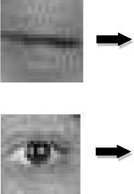
In this method, mean intensity of the eye image is calculated and used as a feature. The basic idea behind using this feature is that, the iris will be darker than the skin area in an image. When the eye is closed, the iris region will be covered by the skin and hence the mean intensity will be higher. When the eye is open the iris will be visible and as a result the mean intensity will be lower. So the mean intensity of eye image varies when eye is closed and open. For extracting the feature the eye image is first resized into size 24×24 pixels and then divided into nine sub regions of size 8×8 pixels each as shown in the Fig.1.

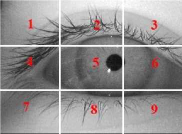
Fig.1. Eye image divided nine sub regions for mean intensity extraction

The mean of the intensities of the pixels in each sub region is then calculated and used as a feature value. So a total of nine feature values are extracted from each image.

• 3)    HOG features

  HOG features [13] were developed by Dalal and Triggs in 2005. It is a commonly used feature based on gradients, and is utilized for object recognition in many computer vision applications.

For the extraction of HOG features also, the eye images are first resized into 24×24 pixel size. Then the images are divided into blocks of size 16×16 pixels with 50% overlap. Thus there are 2 blocks horizontally and 2 blocks vertically. Then each block is divided into four equally sized smaller units called cells with each cell of size 8×8 pixels. Fig.2 shows the cells and the overlapping blocks on an eye image from which the HOG features are extracted.

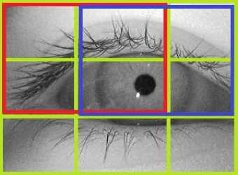
Fig.2. Individual cells (green blocks), overlapping blocks (red and blue blocks)

Then from each cell the HOG feature values are extracted as described below:

First to extract gradient vectors in both x and y direction of each pixel, horizontal and vertical Sobel filters are used:

Horizontal filter, F×= [-1 0 1](6.a)

Vertical filter, Fy= [-1 0 1] T(6.b)

After that the magnitude and orientation of the gradient vectors are calculated using the following equations:

Magnitude: 5 = FP^ + py(7.

Orientation : 0 = arctan

^f Fl 1

I F x J

(7.b)

Once these values are calculated they are quantized into a nine bin histogram. The values of these nine bins will be the HOG feature values extracted from each cell. Similarly, the HOG features are extracted from each cell in each block. So the total number of HOG feature values extracted from each eye image of size 24×24 pixels will be 144. These HOG features extracted from the image are applied to the binary classifier for classification.

• 4)    SVM classifier

  The concept of Support Vector Machine was first developed by Vapnik and his team in 1963 [14]. SVM is a supervised learning algorithm that uses a maximum margin hyper plane to linearly separate between the data into different classes. If, the data is not linearly separable, it is first mapped in to a higher dimensional plane using a kernel function where the data becomes linearly separable. Then an optimal hyper plane is found out in that feature space that linearly separates the data.

Let equation (8) represents a hyper plane that separates two classes of a linearly separable data in a 3 dimensional feature space.

y=m₀+m₁v₁+m₂v₂+m₃v₃ (8)

where y represents the output class and v i represent the feature attributes and the four weights m 1 ,m 2 ,m 3 ,m 4 are the parameters that define the hyper plane. The weights are obtained using a learning algorithm [14]. Then the maximum margin hyper plane is represented in terms of support vector machines are given using the following equation.

У = c + ^ ^a j y j V ⁽ j )(.) v (9) j = 1

where y j represent the class of the training data value and (.) denotes the dot product, v represents the test data and v(j) represent the support vectors. The values c and α i defines the hyper plane. The support vectors and the parameters c and α_i are found out by solving it as a Lagrange optimization problem using Lagrange multipliers.

As mentioned in the beginning of section III.5, in case the data is not linearly separable then it is mapped into a higher dimensional space to find the maximum margin hyper plane and then equation (9) becomes:

y = c + ^ a j L j W ⁽ v ⁽ j ), v ) (10) j = 1

where W() is defined as the kernel function. In this work, a Gaussian radial basis function is used as the kernel function. A detailed discussion on support vectors Machines can be found in [15].

• 5)    Artificial Neural Networks

  The ANN [16] had its beginning when McCulloch and Pitts presented the first artificial neuron in 1943. The ANNs were developed as a result of studies conducted to imitate the working of human nervous system. The working of these computer algorithms is based on learning from examples just like human beings.

A Multi Layer Perceptron (MLP), which is a feed forward neural network trained using back propagation algorithm is the ANN used in this work. The Fig.3 shows the structure of the MLP neural network used here. It has 3 layers of neurons the input layer, the output layer and one hidden layer. The features extracted from the eye image are applied to the input layer. The number of hidden layer neurons is determined using trial and error method. The output layer is binary neuron which gives two values, 0 or 1, representing a closed eye class and open eye class respectively.

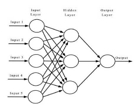
Fig.3. Structure of an artificial neural network

The functioning of ANNs consists of two stages: the training stage and the testing stage. In the training stage, the ANN is trained using the features extracted from a set of known eye images of both the open and closed classes. In the testing stage, this trained ANN is used for classifying an eye image into either of the two classes.

• IV.    Data Bases

• 1)    CEW Database

  The Closed Eyes in the Wild (CEW) [17] was created with the aim of providing a database for testing the accuracy of eye blink detection algorithm in real world conditions. The database consists of eye images extracted from images taken in real world unconstrained environments. It has eye images from 2423 subjects. The images of 1192 subjects are taken from internet and have both their eyes closed. The rest of the eye images of 1231 subjects are taken from Labeled face in the wild (LFW) [18] database. The size of each eye image is 24×24 pixels. The Fig.4 shows a sample of the database used.

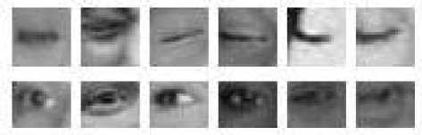
Fig.4. Sample of CEW database used

• 2)    ZJU Eye blink Database

The ZJU [19] eye blink data base consists of eye blinking images of 20 subjects with and without glasses. The images are collected in an unconstrained indoor environment without any special lighting control. The images are taken using a consumer grade web camera. The Fig.5 below shows the sample of eye images obtained from ZJU eye blink database.

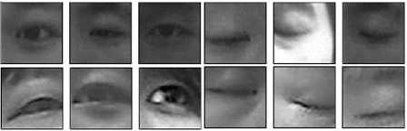
Fig.5. Sample of ZJU database used

• V.    Results And Discussion

Based on the features and classifiers mentioned in section III this paper presents five methods for eye blink detection such as: (i) Fisher Faces with Euclidean distance based classification (ii) Localized Mean intensity with SVM classifier (iii) Localized Mean intensity with ANN classifier (iv) HOG features with ANN classifier (v) HOG features with SVM classifier.

In Method 1, the training images in both the open and closed eyes classes are projected into the Fisher space using the projection matrix given in equation (5). When a new test image arrives, it is also projected into the Fisher space. After that, the average Euclidean distance between the projected test image and the projected images of the training database is calculated. The test eye image is classified into the class of the image, which has the shortest average distance with the test image. Fig.6 shows a sample image of a closed eye class and the average Euclidean distances between the open and closed eyes class. Each of the classes contains 40 images in the Fisher feature space. The mean of Euclidean distance between the closed eyes class is 76.4077 while that with open eye class is 328.1480. Thus, these distances illustrates that the sample image is nearer to closed eyes class. Therefore it is classified as belonging to the class of closed eye.

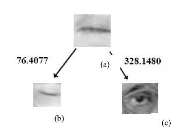
Fig.6. Average Euclidean Distance between closed eye image and images of either class in Fisher space. (a) Test eye image of closed eye (b) Eye image in closed eyes class (c) Eye image in open eyes class

The table 3 shows the mean Euclidean distances between four different sample test images and the training images from both the classes. Based on the minimum distance the test images are classified as shown in the table.

Table 1. Classification of eye images based on Mean Euclidean Distance between test eye images and training images of either class

Sam ple No.	Test Sample Type	Mean Euclidean Distance between Test Sample and		Test Sample is classified into
		Open Eyes Class	Closed Eyes Class
1	Closed Eye	328.148	76.4077	Closed eye
2	Open Eye	39.5431	133.7703	Open Eye
3	Open Eye	21.5828	79.8717	Open Eye
4	Open Eye	45.8252	311.214	Open Eye

From Fig 6 and Table 1 it can be seen that there is a large difference between the projected test image and the projected training images of open eye class if the image belongs to closed eye class and vice versa. The test image is classified to the category which has the minimum distance.

In Methods 2 and 3, the Localized Mean Intensity is calculated by averaging the pixel intensities in each of the nine regions as explained in section III. Fig.7(a) and 7(b) illustrates the Localized Mean intensities of each region of closed and open eyes images respectively. Each cell in table shows the mean intensity of the corresponding sub region of eye image of size 8×8 pixels. When eyes are closed the mean grey levels in central regions 4, 5, 6 is found to be less than other regions. This is due to the presence of the closed eye lids. While for an open eye, the mean grey level drops only in the central region 5 because of the occurrence of the eye ball.

(a)

(b)

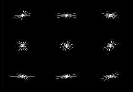
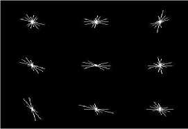
Fig.8. HOG feature vectors of sample images of open eyes (7.b) and closed eyes (7.a). The HOG feature vectors extracted from each of the 9 cells is represented as a vector plot in the image

In Methods 3 and 4 the artificial neural network used is the Multi Layer Perceptron (MLP). The table 2 shows the number of layers and number of neurons in each layer for each method.

(a)

Fig.7. Localized Mean Intensities in each region of sample images of open (7.a) and closed eyes (7.b). Each cell in the table represents the mean intensity of the pixels in that sub region of size 8×8 pixels.

129.0	145.0	133.9
102.0	105.0	97.9
128.0	124.9	128.0

Table 2. Number of hidden layers and neurons used in ANN for each method

Method	HOG-ANN	Localized Mean intensity- ANN
No of Layers	3	3
No of input Layer Neurons	144	9
No of Output Layer Neurons	1	1
No of Hidden Layer Neurons	200	100

(b)

159.9	152.9	142.9
157.9	83.9	122.9
155.0	152.0	153.0

To evaluate the performance the accuracy of each method were calculated. For this, the classifiers were trained using 160 images, 80 images each of open and closed eyes. 40 images taken from CEW database were used for testing the accuracy of these methods. These images taken in real world unconstrained environments. The test database consisted of 10 images each, of closed left eye, open left eye, closed right eye and open right eye.

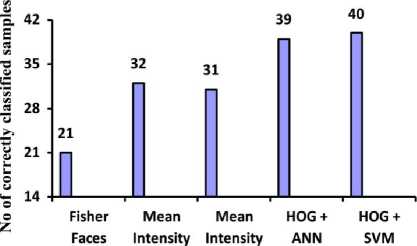
The test results are plotted in the bar graph given in Fig.9. Each vertical bar represents the number of correctly classified sample out of the 40 test images for the five different methods.

In Method 4 and 5, involving HOG features, a total of 144 feature values are extracted from each of the eye image. These features are then utilized for classifying the eye image. The Fig.8 shows the representation of HOG feature vectors extracted from the open and closed eyes. Each vector plot in the image represents the HOG feature vector extracted from the corresponding cell in eye image. Each of the nine vector plots represents the HOG feature vector from each of the nine 8×8 pixel cells of the eye image.

+ SVM +ANN

Fig.9. Number of correctly classified samples in each method

The accuracy of each method is tabulated in table 3.

The accuracies obtained are tabulated in table 6.

Table 3. Accuracy of each method when tested on 40 images

Method	Accuracy
Fisher Faces	52.5%
Mean Intensity +SVM	80%
Mean Intensity +ANN	77.5%
HOG+ANN	97.5%
HOG+SVM	100%

From the table 3 it can be seen that the combination of HOG features with SVM classifier gave the highest accuracy while the Fisher faces provided the least accuracy. In Fisher Faces method, no classifiers were used. Only the value of minimum Euclidean distance was used to find out, to which class the test image belong to.

In order to further evaluate the performance of HOG features with SVM classifier method, the number of training images was varied and the accuracy was computed. A good practical classifier provides better accuracy rate even with smaller training sets. Four different datasets were prepared to train each of the methods presented. These training datasets were used to measure variations in the performance of these methods when the number of training images is changed. The table 4 shows the details of each training dataset.

Table 4. Four different datasets generated for training each of the methods

Dataset	No: open eye (left/right)	No: closed eye (left/right)	Total images
Set80	20/20	20/20	80
Set120	30/30	30/30	120
Set160	40/40	40/40	160
Set200	50/50	50/50	200

Dataset Set80 means that it contains a total of 80 images, with 20 images each belonging to open left eye, open right eye, closed left eye and closed right eye class. Similar is the case with Set120, Set160 and Set200. Each of these datasets was used to train each of the methods separately. These trained classifiers were then tested using another set of 40 eye images, 20 images each of open and closed eyes, which were not included in the training sets. Results are tabulated in table 5

Table 5. Number of correctly classified samples, when each method is trained with different number of training images

Dataset used for training	Fisher Faces	Mean Intens ity + SVM	Mean Intensity + ANN	HOG +ANN	HOG+ SVM
Set80	17/40	32/40	32/40	30/40	40/40
Set120	21/40	33/40	31/40	38/40	40/40
Set160	21/40	32/40	31/40	39/40	40/40
Set200	17/40	33/40	32/40	39/40	40/40

Table 6. Accuracy of each method when trained with different no of images in the training dataset

Dataset used for training	Fisher Faces	Mean Intensity + SVM	Mean Intensity + ANN	HOG +ANN	HOG+ SVM
Set80	42.5%	80%	80%	75%	100%
Set120	52.5%	82.5%	77.5%	97.5%	100%
Set160	52.5%	80%	77.5%	97.5%	100%
Set200	42.5%	82.5%	80%	97.5%	100%

The Fig.10 compares the accuracy of each method when the number of training images is varied. All methods except the HOG-SVM method showed variation in accuracy when the number of images in the training dataset is varied.

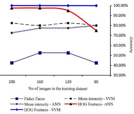
Fig.10. Plot of accuracy of each method for Different training sets

From the above results, it was found that, the combination of HOG features with SVM classifier provided highest accuracy in detecting the eye blinks with less number of training images.

Statistical Analysis: A statistical analysis of the performance of HOG-SVM classifier was also conducted. For this, a database whose images are captured under a wide range of lighting condition with low resolution was used. 800 images taken from the ZJU database, out of which 400 images were of closed eyes and the rest of the 400 were of open eyes. The closed eyes images are also referred to as eye blinks in this analysis. Results obtained are given in table 7 in the form of the confusion matrix [20] of the classifier. The confusion matrix helps to identify if the classifier is confusing between the two classes. From the confusion matrix it can be seen that out of 400 images 299 images of the closed eyes were correctly classified as the blinks and 386 open eye images were classified as open by the classifier. While 14 of the closed eye images and 101 open eye images were classified into the wrong class by the classifier.

Table 7. Confusion Matrix of HOG-SVM classifier

Predicted	Actual
	Blink	Open eyes
Blink	299	101
Open eyes	14	386

In this classifier, classifying into closed eye class is considered as positive while classifying into open eye class is considered as negative.

True positive defined as the number of closed eye samples that are correctly classified as blinks and true negatives are the number of open eye samples that are correctly classified as the open eyes. Similarly the false positives are the open eye images that are wrongly classified as blinks and false negatives are the closed eye images wrongly classified as open.

From the confusion matrix the parameters precision, recall, specificity and accuracy [21] were calculated using the following equations.

true negative Specificity = false positive+true negative true positive Precision = true positive+false positive true positive

Recall rate = true positive+false negative true positive+true negative Accuracy =

Total number of classified samples

The values of these parameters were calculated

(14) from

the confusion matrix. It can be seen that HOG-SVM classifier has a specificity of 79.26%. It denotes the classifiers ability to detect open eye images. It is a measure of the ratio of the number of images that were correctly classified as open eye out of the total number of open eye samples. The recall rate of the classifier is 95.52%. It is the measure of its ability to correctly classify the closed eye images as blinks. The precision of the classifier is 74.75% that denotes the percentage of closed eye image predictions that were correct. Finally the classifier has a total accuracy of 85.62% which is the overall performance of the classifier and the measure of its ability to correctly classify the samples to either of the classes. Thus the HOG feature based SVM classifier proved to be efficient with an overall accuracy of 85.62% when tested with a totally unknown database.

The accuracy of the presented HOG+SVM method was then compared to some of the existing methods available in the literature. The table 8 compares the accuracy of the presented method and existing methods. The table 8 illustrates that CEW database which contain real world images gave an accuracy of 100%. While testing with ZJU database, which contained low resolution images, this classifier gave an accuracy of 85.5%.

Table 8. Comparing the HOG-SVM method with the existing methods

Other Methods	Accuracy
Google Glass method [9]	67 %
Template matching (poor illumination) [7]	77.2%
Component based model [25]	79.24%
Gabor features + NN [17]	85.04 %
Hybrid model based method [23]	90.99%
Gabor features + SVM [17]	93.04 %
Intensity vertical projection [5]	94.8%
Template matching [24]	95.3%
Template matching (good illumination) [7]	95.35 %
SIFT feature method [6]	97%
Presented method (HOG+SVM)
In ZJU Database	85.5%
In CEW Database	100%

• VI.    Conclusion and Future Scope

In this paper, five methods for detecting closed eye or eye blinks by combining different features extracted from eye images and different classifiers were presented. Among these five methods, HOG features combined with SVM classifier showed extremely high performance in comparison to other methods. It gave the highest accuracy of 100% when tested with low resolution real world images from the data set used for training and gave an accuracy of 85.62% when tested with images from an entirely different dataset taken in completely unconstrained indoor environments without any lighting control. It could also successfully detect eye blinks with an accuracy of 100% even when trained with less number of training images.

The developed method of eye detection can be integrated into various systems and used for a wide variety of applications. The eye blink detection can be used for drowsiness detection, concentration level estimation, behavioral analysis, physiological studies and so on.