Non-parametric identification and control algorithms for T-processes

At present, the problems of identification and control of multidimensional discrete-continuous systems with a delay under conditions of a priori uncertainty are quite important [1]. In many productions, processing and storage industries, technologists usually deal with multidimensional discrete-continuous processes. For example, complex physicochemical reactions occur during the production of converter steel, and therefore the lack of an adequate model can lead to unsuccessful control of the converter, associated with a large difference (more than 5%) of the values of the output variables from the set ones. In this case, the construction of a parametric model of converter production will lead to more experiments and, accordingly, to numerous costs, while the use of nonparametric models significantly reduces costs and reduces the time to create an adequate model [2].

Such multidimensional objects (processes) most often have dependencies of output variables x = (x1,x2,...,xn ), stochastically dependent in an unknown way in advance (T-processes). This leads to the fact that the mathematical description of a multidimensional object will be presented in the form of some analogue of a system of implicit functions of the form Fj (u, x) = 0, j = 1, n, where u = (u1, u 2,..., um ) are the input variables of the process. The main feature of such objects is that the de- pendency class is F (•) unknown up to the parameters. In this case, the classical theory of identification is not applicable. The identification problem is reduced to the problem of solving a system of nonlinear equations with Fj (u, x) = 0, j = 1, n respect to the components of a vector x = (x^, x2,—, x„ ) with known values of u, x and the presence of a training sample (ui, xi, i = 1, s), which can be solved using the theory of nonparametric systems [1]. Similar tasks have not been considered before [3; 4].

Use the concretization of the concept associated with the term "nonparametric", which was used in the works of M. Rosenblatt and E. Parzen [5; 6], as well as in the monograph of F. P. Tarasenko [7].

«A nonparametric problem is a statistical problem defined on such classes of distributions, among which at least one is not reduced to a parametric family of functions. »

«The nonparametric problem of estimating unknown distributions is the problem of finding a procedure by which one can evaluate nonparametrized distributions from a class, for example, of all continuous distribution functions or a class of distributions having a number of derivatives, etc. »

In the present article, the term «nonparametric» means the lack of sufficient a priori information to represent an object with accuracy up to parameters.

Based on these definitions, we can say that nonparametric methods are much more effective if the parametric model does not adequately describe the observed data [8].

Identification task

Consider the multidimensional process shown in fig. 1.

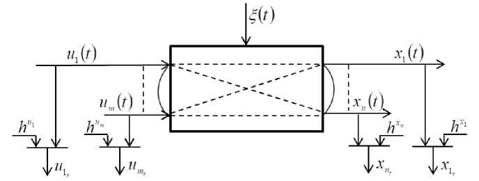
Fig. 1. Multidimensional object

Рис. 1. Многомерный объект

In fig. 1 given the following designations: u ( t ) = ( u 1 ( t ) , u 2 ( t ) ,..., u k ( t ) ,..., u m ( t ) ) , k = 1, m m -dimensional vector of input variables; x ( t ) = ( x 1 ( t ) , x ₂ ( t ) ,..., x j ( t ) ,..., x_n ( t ) ) , j = 1, n - n -dimensional vector of output variables, which belong to the respective areas: x j - eQ j ( x ) ; ^ ( t ) - random noise acting on the object; h^u , h^x – random noise measurement of relevant process variables; the dotted lines indicate the presence of the input and output variables; ( t ) is a continuous time; u , x – measure the input and output variables in discrete time t .

Based on the above, we can say that multidimensional processes surround our daily life and are processes that have many inputs and outputs, as well as connections between input and output variables, connections only between input variables [9; 10] and only between outputs. Moreover, all these connections are not always known to the researcher [11], and there may also be different types of a priori information [12]. Because the output variables of a multidimensional process are interconnected, it should also be noted the composite (situational) vector that was introduced by Ya. Z. Tsypkin in [13]. A composite vector is a vector composed of input and output variables. It can be any set, for example x<3> = (u2, u5, ^, x4).The composite vector is known to the researcher from a priori information.

Consider the concept of lag in a multidimensional object. In one case, the lag is a natural property of the object (for example, it may be the duration of the clinker grinding process to obtain cement). In another case, the delay will be related to the discreteness of measurements, for example, if the output characteristics of a process or object can be observed only after a certain period. Thus, in control theory, lag and delay should be distinguished in different ways. It should be borne in mind that the delay may depend on the equipment and measurement technology, when measurements of output variables are carried out at different time intervals, for example, once every two hours, once a shift, once a day, etc.

The task of identifying multidimensional objects is to build models of these objects, which can be conditionally represented in fig. 2.

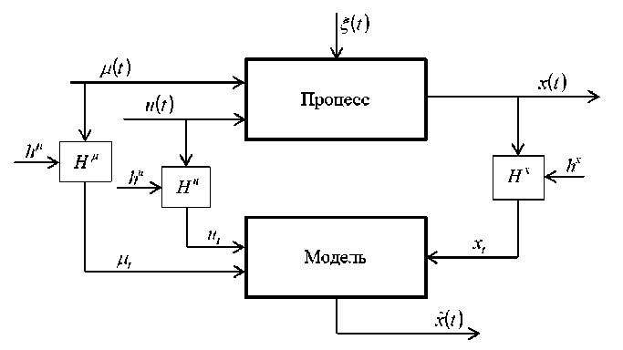
Fig. 2. Multidimensional discrete-continuous process

Рис. 2. Многомерный дискретно-непрерывный процесс

In fig. 2, the input of the process under consideration receives a vector of input controlled variables u ( t ) = ( u ( t ) ,...u_m ( t ) ) e ( u ) ^c R m and a vector of input unmanaged, but controlled variables ц ( t ) = ( ц 1 ( t ) ,... Ц p ( t ) ) е ( ц ) с R^p , at the output there is a vector of output variables x ( t ) = ( X j ( t ) ,... x_n ( t ) ) e ( x ) c Rⁿ , x ( t ) - model output. The input and output variables are monitored at discrete time with intervals A t . By means of control, we H^u , H ^ц , H^x get a sample of observations or a training sample. Random interference occurs in the measurement channels of variables h^u , h ^g , h^x .

As mentioned above, the processes considered in this paper have unknown dependencies of the components of the output variables. Therefore, the process under study will be described by a system of implicit stochastic equations:

F j ( u ( t ) , ц ( t ) , x ( t + t ) , ( t ) ) = 0, j = 1, n ,

where the functions F j ( • ) are not known, since the dependencies of the output variables are not known; т - known lag through various channels of the process under study.

The identification task consists in constructing a model of the system, which is shown in Fig. 2, in the presence of a sample of observations over the object: u i = ( u i1 , u i 2 , ..., u im ) , M i = ( m i 1 , M i 2 , -, M ip ) ,   x i = ( x i 1 , x i2 , -.., x in ) ,   i = 1, ⁵ .

In this case, the T-model of the process with unknown dependencies of the components of the vector of output variables will be considered as a system:

F i ( u < j > , M < j > , x < j > , u . , M 5 , x_s ) = 0, j = 1, n ,                               (2)

where u < ^j > , ц < ^j > , x < ^j > are composite vectors u_s , ц ₅ , x_s - are time vectors (i.e., a set of data that arrived at the s -th moment of time).

As a result of measuring input and output variables, a training sample can be obtained u i = ( u n , u_t 2 , ..., u 'm ) , M i = ( m i 1 , M i 2 , ..., M ip ) , x = ( X i 1 , x i ₂ , •••, ^x in ) , i = 1, s , which is used when building a model of a multidimensional object. Since the input effects u are set and known, we solve the system (2) and obtain estimates of the x ˆ _j components of the vector of output variables x_j at the corresponding values of the input effects u . Here we will use nonparametric estimation methods [14].

To begin with, we substitute the l -th receipt of input variables u_l = ( u_l 1 , ..., u_lm ) , l = 1, s , where s is the volume of the training sample, into the formula (2). Next, we substitute the output variables from the training sample x i = ( x i 1 , ..., x_n ) to determine the residuals 8 i , i = 1, s . The residuals 8 i , i = 1, s are calculated using the following formula:

⁸ ij = ^fJ ( u < ^j > , M < ^j > ’ x < ^j > , u s , ^M s , x s ) , j = 1, ⁿ , ⁽³⁾

where the functions  fj (•) are taken as the difference between the measured values of the output components and their estimates [15]:

8,-

⁽ i ) = x j ⁽ i ^)-

s      <  m >

Z x j [ i 1 П Ф i = 1         k = 1     к

'           <  p > Л

■     п Ф csuk    J V=1   к

^{MV   MV [} ' ^]

C...

^{s M}V     J

s <  m >   (

Zn Ф i = 1 k = 1     к

u     '

c^suk    J

< p >  Л

П ф

^V = 1    к

^{Mv   Mv [} i ^]

C ll ^{s M}V    J

j = 1, n ,

where <  m >  is the dimension of the composite vector u_k , <  m ><  m.

Next, we evaluate the conditional mathematical expectation xj = M {xj | u , M, 8 = 0} , j = 1, n,

and in the end, the forecast for each component of the vector of output variables will look like this:

x j =

V г-i < Г > /tsf u ki   uh ^[ i ¹'y p r rbf^M vi    ^M v| ^[ i ^] ' < — > ^f⁸ k 2 ^[ i ^]

Z x j [ i ] ’ П ^ф — П ^ф — П ф ² i = 1         k 1 = 1    к      c su     J v 1 = 1    к      ^Cs M       J k ₂ = 1    к   c s 8   J

>■ < m > zn Ф

Г ukL

-M i l 1

i = 1 k 1 = 1 к

C su     J

< p >

Пф v1 =1

^Mv 1

^{M 1} i ¹ 'I n ф ■ k 2 ^[ i ¹

^Cs M     J k 2 = 1 к   ^Cs 8   J

j = 1, n ,

where Ф ( • ) functions of various types were taken as bell-shaped functions and the coefficients c , c , c satisfied the convergence conditions [16].

Estimate (6) is a prediction of output variables x with known input u .

Management task

Consider a multidimensional object – a block diagram with a lag, the general control scheme of which is shown in fig. 3.

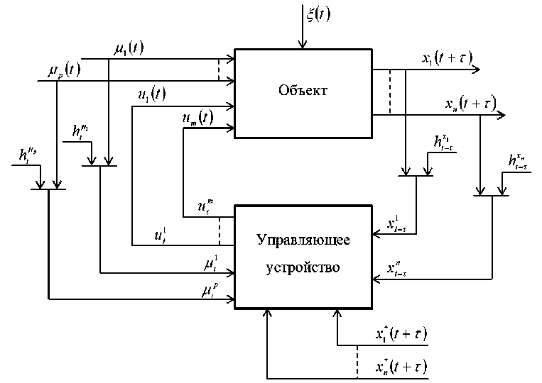
Fig. 3. Scheme of a nonparametric control system for an object with a lag

Рис. 3. Схема непараметрической системы управления объектом с запаздыванием

In fig. 3, the following designations are adopted: u(t) = (щ (t), ..., um (t)) - controlled input vari- ables

(ц1 (t), ..., цp (t))   - uncontrolled, but controlled input variables - x(t + t) = (Xj (t + t), ..., xn (t + т))еRn          -          output          process          variables;

x (t + t) = (x* (t + t), ..., xn (t + t)) e Rn - setting influences - ^t, ЬЦ, htx - random stationary inter ference acting on the object and in the measurement channels of input and output variables - t - lag on various channels of a multidimensional system. The lag t is known across all channels of the multidimensional system, and in this case, it is the same for each component of the vector of output variables.

Taking into account that the output variables of a multidimensional T-process are stochastically interconnected, and then the definition of the driving influences for such a system acquires some difference. Since the output variables are connected, they have a common intersection in some area Qj (Xj), but not always all output variables will intersect in one area. In the event that this area Qj (Xj) exists, then the setting influences must be selected only from this area, otherwise it is not possible to control such a system. If there is no such area, then it is useless to manage such a system. At the same time, we present a control system for a multidimensional object, in which we consider a system of interrelated setting influences (fig. 4).

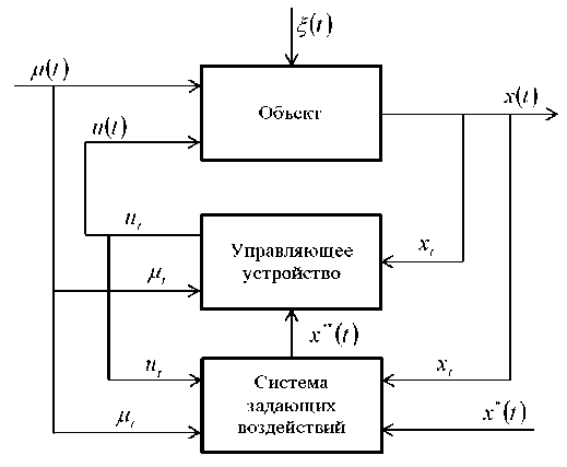
Fig. 4. Diagram of a nonparametric control system with an additional block

Рис. 4. Схема непараметрической системы управления с дополнительным блоком

Fig. 4, in contrast to fig. 3, is supplemented with a block for the formation of setting influences for their determination. In fig. 4, the following designations are adopted: x * ( t ) - the initial values of the setting effects; x ** ( t ) - the setting effects that need to be found from the system of equations

F j ( u < j > ( t ) , ц < j > ( t ) , x *< j > ( t ) ) = 0, j = 1, n ,

where functions F j ( • ) continue to remain unknown. Outline the control procedure starting from a specific moment in time t .

Let there be a training sample ( u i , ц i , x i , i = 1, s ) . At a specific moment of time t , unmanaged but controlled variables are received at the input ц _t , while the control actions u_t and output variables are x_t still unknown. Then, from the entire initial sample ( u i , ц i , x i , i = 1, s ) , those rows are selected in which the values ц i are closest to the newly received values ц _t ,and a new sample is formed from these rows. The setting influences x ** are found from the newly formed sample x * * e A ( x j ) , namely from the solution of the system (7). The solution of system (7) is reduced to the sequence of algorithms described below.

For the setting effect x *** , we take random values from the region Q 1 ( x 1 ) . The second variable x 2* is defined taking into account the selected component x₁ '* from the following expression:

x 2 ** ¹

s ₁

I x 2 Ф

1 = 1

**

^x 1

c

^x 1

x ₁

< m >

s ₁

I Ф

1 = 1

**

^x 1 •

c

^{— x} 1

7 k = 1

< m >

uk uk cuk

< p >

Ц у

—

Ц у

c s Ц

x j     7 k = 1

^uk ^{— u}k c_{u k}

< p >

Ц у

—

Ц у

c s Ц

where S j cQ ( x^ ) , i. e. the summation is not carried out for the entire initial sample, but only for those values that were closest to the newly received values Ц _t .

In general, the algorithm takes the following form:

„** s x_j

s j —1     j — 1

I x j П i = 1      j = 1

х, — x

c

j П Ф k=1

^uk ^{— u}k c u_k

П

7 ^V = 1 к

Ц у

—

Ц у

c s Ц

.

s j —1 j — 1

х, — x

c

j П Ф k=1

^uk ^{— u}k c u_k

П

7 ^V = 1 к

Ц у

—

Ц у

c s Ц

After determining the setting effects, you can start finding the predicted values of the control effects for a multidimensional system. To do this, we use the following nonparametric algorithm. We take the input variable щ ( t ) arbitrarily from the domain Q ( щ ) . The input variable u ₂ ( t ) can be determined according to the following algorithm:

s

I щ ²Ф

1 =1

^u 2 =------7

s

I Ф

¹ =1 к

ui   ui cu1

u 1 — u 1

c u

n

П Ф

n

П Ф

**       1

x,- — x_;

c

p

П Ф

Ц у

—

ц V

c Ц v

**       1

x,- — x,

c

p

П Ф

Ц у

—

ц V

^C Ц v

where ( u¹ , ц ¹ , x¹ , 1 = 1, s ) - training sample; ц_у - incoming input unmanaged, but controlled variables.

For the input variable u 3 ( t ) , the control algorithm will look like this:

s

I u / Ф

1 = 1

u 3 =------ s

I Ф

1 = 1

_„1 Л ^u__u 1

к   ^cu 1

< u__u1

Ф

Ф

к   ^cu 1    7

_„1 Л u 2 u 2

к   c^u 2

i u2 u2

к   c u 2

n

П Ф

7 j = 1

n

П Ф

7 j = 1

**

x, — x

i

p

c

i

j П Ф

Ц у

—

ц V

**        1

x, — x

^C Ц v    7

,

p

c

j П Ф

Ц у

—

ц V

^C Ц v

and so on for each input component of the u ( t ) object. In general, for a multidimensional system, the control algorithm will look like this:

^us ^k

s     k — 1

I u k п ф

1 = 1      k = 1

s k — 1

In Ф

1 = 1 k = 1

i uk— uk

к   c^uk

i uk  uk

n

П Ф

**

x, — x

c

11-      P

- ПФ

V= 1

Ц у

—

1 л

Ц<

c к  cuk

n

П Ф

**       1

x,- — x

c

1 ■ p j ПФ

V= 1

к

ЦV

c Ц v

—

i

ЦV

—, k = 1, m .

к c Ц v   7

In real tasks, the number of components of the vector of input variables u is often greater than the number of components of the vector of output variables x . In this case, the components of the vector u , are included in the number of the components vector ц , so that the dimension of the vector u and x to be the same.

The configurable parameters will be the blur parameters c ,

c x j ^and с ц_v ,

the following formulas

can be used for them: cuk = a\uk - ulk ,  cx. = p|x** -xi andc^v = у|цу -цV|, where a, pand ysome parameters are large 1, a> 1, > p> 1, > y> 1. It should be noted that the choice cuk, cx and c^ is car ried out on each control cycle. At the same time, if it is first defined c ,, then the definition c с is uk                               xj    цу carried out taking into account this fact. However, it may be the other way around, for example, it is determined first c or с ,and then the rest.

^x j      ^Цv

Computational experiments

For example, an object with 4 input variables u ( t ) = ( u_x ( t ) , u ₂ ( t ) , u ₃ ( t ) , u ₄ ( t ) ) and three output variables was taken x ( t ) = ( x _t( t ) , x ₂ ( t ) , x ₃ ( t ) ) . Such objects are typical for real industries, for example, for cement production, oil refining, metallurgy, etc., where only multidimensional processes take place. A sample of input and output variables was formed for this object and the predicted values of output variables were found for known input variables using algorithm (4) and (6). To calculate the sample size, s = 1000, the blur parameters c_su = 0,4; c_S£ = 0,2, the interference acting on the components of the vector of output variables a = 0,1, the lag т = 2 of the cycle (where 1 clock cycle is equal to 1 minute or another) were used. The description of the object up to the parameters was accepted only for the computer research and remained unknown for the theory outlined above. Present the results obtained for the third component of the output of a multidimensional object.

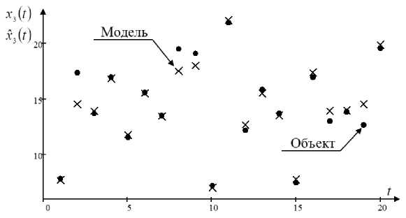
Fig. 5. The predicted output variable x 3 ( t ) of the object, measured with a uniform noise of 10 %, 5 3 = 0,07

Рис. 5. Прогноз выходной переменой x 3 ( t ) объекта, измеренный с равномерной помехой 10 %, 5 3 = 0,07

Figure 5 shows the predicted values obtained x3 (t) for the third component of the output x3 (t). Errors in determining variables are caused by the presence of interference. As can be seen from Fig. 5, the prediction of the values of the output variables x3 (t) of a multidimensional object based on known input variables u (t), taking into account 10% interference, is quite satisfactory from the point of view of many practical tasks (for example, the clinker grinding process). The attention should be payed again to the fact that the researcher does not know the type of system of equations describing the controlled object. Measurements of input and output variables are used as information about the last. (ui, цi, xi, i = 1,s).

The following are the results of computational experiments for this object for the first component of the output using the control algorithm (12). In this computational experiment, the number of components of the vector u is greater than the number of components of the vector X. If the dimension of the vector u exceeds the dimension of the vector x , i.e. m >  n , then we will replace u ₄ ( t ) ^ ц ( t ) to make the dimension of the vector u and x the same. Further, the values of the setting influences x *** ( t ) , that were found using the algorithm (9) are presented in the form of a step function, as shown in fig. 6.

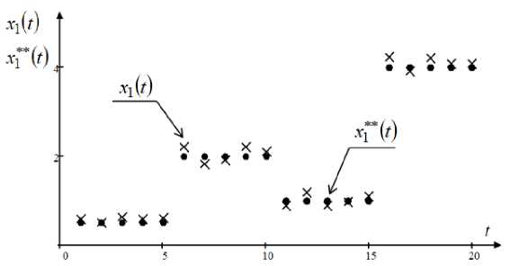
Fig. 6. Dependence of the output of the object X 1 ( t ) on the setting action x ** ( t )

Рис. 6. Зависимость выхода объекта X 1 ( t ) от задающего воздействия x “( t )

As can be seen from Fig. 6, the output of the object x 1 ( t ) is close enough to the setting effect x ** ( t ) in the presence of 10% interference and does not exceed 1.7% of the values x ** ( t ) ,, which satisfies most practical tasks.

Thus, a nonparametric algorithm for controlling a multidimensional object with stochastically dependent output variables x ( t ) shows accurate results from the point of view of many practical problems.

Conclusion

This article discusses the problems of identification and management of a multidimensional object in conditions of incomplete information about the object of study, i.e. in conditions when the parametric model of the process is not defined. Such multidimensional objects are often found in practice, for example in metallurgy, energy, oil refining and other industries. A distinctive feature of the models of these objects and algorithms from the known ones is that the tasks are set in conditions of nonparametric uncertainty, i.e. in conditions when a multidimensional system is not described with accuracy up to the parameter vector due to a lack of a priori data.

Another main feature is that both the identification task and the control task introduce sequences of nonparametric algorithms. The essence of nonparametric identification and control algorithms is that for the identification problem, the forecast is built as a conditional mathematical expectation of the components of the vector of output variables x (t) with known input components u (t),, and in control - as a conditional mathematical expectation of input variables u (t) with the found setting influences x **( t).

Based on the predicted values obtained in the computational experiment, in the process of using nonparametric algorithms, quite good results are obtained from a practical point of view, which can also be used in solving real problems in production [17].