Nonlinear Blind Source Separation Using Kernel Multi-set Canonical Correlation Analysis

Published Online November 2010 in MECS

In recent years, blind source separation (BSS) raises great interest. In fact, BSS plays an important role in many diverse application areas, such as radio communications, radar, sonar, seismology, image processing, speech processing (cocktail party problem) and biomedical signal analysis where multiple sensors are involved. In the last years, linear BSS has become relatively well established signal processing and data analysis techniques [1]. On the other hand, nonlinear BSS is technique that is still largely under development, and has the potential to become rather powerful tools [2].

Kernel-based methods have also been considered for solving the nonlinear BSS problem [3], [4]. The data are first implicitly mapped to high-dimensional feature space, and the effective reduced feature space in feature space is extracted, translate the nonlinear problem in the input space to a linear problem in reduced feature space.

Canonical correlation analysis (CCA) is a classical tool in multivariate statistical analysis to find maximally correlated projections between two data sets, since it was proposed by H. Hotelling [5]. There are detail descriptions of CCA in [6], which has been widely used in many modern information processing fields, such as for test of independence [7], blind equalization of MIMO channels [8] and BSS [9],[10]. With CCA, the objective is to find a transformation matrix which is applied to mixtures and maximizes the autocorrelation of each of the recovered signals (the outputs of the transformation matrix). By maximizing this autocorrelation, the original uncorrelated source signals will be recovered. This approach rests on the idea that the sum of any uncorrelated signals has an autocorrelation whose value is less or equal to the maximum value of individual signals [11]. The algorithm based on CCA which computation burden is little and the flexibility is strong, can satisfy the demand of engineering application. Based on the idea of maximize generalized relativity measurement, J. Kettenring present-ed several ways to generalize CCA to more than two sets of variables, namely MCCA (Multiset CCA) [12]. By assuming that sources are not correlated with the others and every source has a different temporal structure, which is a mild condition that can be easily, satisfied in practical applications, a MCCA linear BSS algorithm was proposed in [13]. This paper proposed a novel nonlinear BSS algorithm based on kernel feature spaces and MCCA. The algorithm can adapt to nonlinear BSS with invertible nonlinearity. The details of the new method will be described in the following sections. The paper is organized as follows: Section II presents the detail analysis of linear BSS algorithm based on MCCA. In the Section III, the new nonlinear BSS algorithm based on kernel MCCA will be analyzed. Then some simulations of the algorithm proposed in this paper are conducted in the Section IV. Section V is the conclusion.

• II.    Linear BSS Algorithm Based on MCCA

• A.    Linear BSS problem formulation

Consider the following instantaneous linear mixture model:

x ( t ) = Hs ( t ) + n ( t ).               (1)

where x ( t ) = ( x 1 ( t ), x ₂( t ),L x m ( t )) T ( t = 1,L T ) is the m -dimensional vector of mixed signals observed by m sensors, n ( t ) is the additive noise vector, H is the unknown m x n mixing matrix, s ( t ) = ( s ₁( t ), 5 ₂( t ), L s_n ( t )) ^T ( t = 1,L T ) is the n -dimensional vector of source signals (which is also unknown and m >  n ), and the superscript ^T denotes the transpose operator. BSS methods aim at estimating the source signals s ( t ) . Suppose the source signals are not correlated with the others and every source has a different temporal structure, and the additive noise vector n ( t ) is statistically independent of s ( t ).

The task of BSS is to estimate the mixing matrix H (or is pseudo-inverse, W - H # that is referred to as the demixing matrix), given only a finite number of observation data x ( t ) ( t - 1,L T ) . And obtain the estimated source signals y ( t ) = ( y 1 (t ), y ₂( t ),L y_n ( t )) ^T ( t - 1,L T ) :

y ( t ) = Wx ( t ).                   (2)

We just consider the case of m - n , for less sources than mixtures ( m >  n ) the BSS problem is said to be over-determined, and it is easily reduced to a square BSS problem by selecting m mixtures or applying some more sophisticated preprocessing like PCA.

• B.    MCCA

CCA is a multivariate statistical technique similar in spirit to principal component analysis (PCA). While PCA works with a single random vector and maximizes the variance of projections of the data, CCA works with a pair of random vectors (or in general with a set of m random vectors) and maximizes correlation between sets of projections.

Given two random vectors, x ₁ and x ₂ , of dimension p ₁ and p ₂ . The first canonical correlation can be defined as the maximum possible correlation between the two projections u 1 - a 1^{(1) T} x 1 and v 1 = a 1^{(2) T} x ₂ of x 1 and x ₂ [6]:

P 1 ( x 1 , x 2 ) = max ) corr ( « Г’ T x 1 , ^ ' T x 2 )

α ₁, α ₁

α (1) T C α (2)                   (3)

= max ------------- ¹ 1/ ^{12 1} -----------17

af1’-af2’ (a'1)T C11 a'1))X (a(2)T C22a(2))Л where C11 = x1 xT, C12 = x1 xT, C 21

T x2x1 , V22

= x 2

x ₂ ^T .

After finding the first pair of optimal vectors α1(1) and α1(2) , we can proceed to find the second pair α2(1) and α2(2) which maximizes the correlation and at the same time ensures that the new pair of combinations {u2,v2} is uncorrelated with the first set {u1,v1}. This process is repeated until we find all the min(p1, p2) = p pairs of optimal vectors a™ and a'21, i - 1,2, l , p .

Since the choice of rescaling is therefore arbitrary, Normalizing the vectors α _i ⁽¹⁾ and α _i ⁽²⁾ by letting a® ^T C 11 a ™ = 1 and а*^{2) T} C ₂₂ а *²⁾ = 1 , we see that CCA reduces to the following Lagrangian [6]:

L ( A , a, ⁽¹⁾ , a (²⁾ ) = a ,^{(1) T} Ca - ~( a ,^{(1) T} Ca - 1)

ii i i 12 i 2 i 11 i

- ^ Ч a (^{2) T} C ₂₂ a'²’

^{- 1)}

Taking derivatives in respect to α _i ⁽¹⁾ and α _i ⁽²⁾ , the CCA problem can be obtained by solving the following generalized Eigen values problem

С С-¹С /х⁽¹⁾ — 9 ² С /х⁽¹⁾

C 12 C 22 C 21 ^ai = ^/L i C 11 ^ai

.

Г* Г* ^-1f zi^ — ^f x/²⁾ C 21 C 11 C 12 ai - /Vj C 22 ai

There’s a generalized Eigen problem of the form Ax - A Bx . We can therefore find the coordinate system that optimizes the correlation between corresponding coordinates by first solving for the generalized eigenvectors of (5) to obtain α _i ⁽¹⁾ and α _i ⁽²⁾ .

According to the ways in [6] we can generalize CCA problem to the minimization of the total distance.

For CCA, two matrices A(1) and A(2) contain the vectors (α1(1),L, α(p1)) and (α1(2),L,α(p2)). The CCA problem can also be express as max tr(A(1)TCA(2))

A (1) , A (2)                           12

5 . t .       A ^{( k} ) ^T C kk A ^{( k} ) - 1

a,(k)T Cka (1) - 0 iklj k,I - {1,2},I ^ k,i, j - 1,l,p, j * i

where I is an identity matrix with size q x q .

The canonical correlation problem can be transformed into a distance minimization problem where the distance between two matrices is measured by the Frobenius norm:

min       ll xA ⁽¹⁾ - x₂A ⁽²⁾||

A (1) , A (2)       12 F

• 5 . t .       A ^{( k} ) ^T C kk A ( k ) - 1            .       (7)

• 5 . t .       A ^{( k} ) ^T C k, A ( k ) - 1                    (8)

a <^k ) ^T C_k a (¹) - 0

iklj k, I - {1,2}, I * k, i, j - 1,l, p, j * i

We can give a similar definition for MCCA. Given m multivariate random variables in matrix form { x 1 , l , x _K } . We are looking for the linear combinations of the columns of these matrices in the matrix form A ⁽¹⁾ , L , A ^{( K )} such that they give the optimum solution of the problem:

min V K     ll xA ^{( k} ) - xA ^{(1 )}||

A (1) , L , A ( K )           i—ik , I - 1, k * / II ^k              I       Il f

a ,' k ) ^T C_ka (¹) - 0

iklj k, I -1, l , K, / * k, i, j -1, l , q, j * i which is the sum of the squared Euclidean distances between all of the pairs of the column vectors of the matrices xk A(k), k - 1,l, K .

• C.    BSS Algorithm Analysis

We start by specifying the signal. It is assumed that the sources are spatially uncorrelated, the correlation matrix of the sources R ₅₅ [ t ] - E{ s ( t ) s ^T ( t - т )} is a diagonal matrix, where E{ - } denotes the statistical expectation operator. For nonzero correlation lags, we have

R ss [ г ] = E { s ( t ) s ^T ( t - т )} = diag^ ),L , X m ( t )}      (9)

with X i ( t ) * 0 for some nonzero delays т .

First, we choose the observed signals x ( t ) as x ₁ and x ( t - т ) as x 2 . Then the Eigen value problem in (4) becomes

R ( t ) R m R ( t ) a ™ = X² R xx (0) a^ R xx ( t ) R m R xx ( t ) a (²⁾ = X , ² R xx (0) a (²⁾

where R _xx ( t ) and R xx (0) are the correlation matrices of the mixed signals.

In the context of BSS, the vectors αi(1) and αi(2) in (5) are the same and denote them by wi = a*1) = a'21. Which is the demixing vector applied to the mixed signals. The Separate signals can be obtained yi( t) = wT x (t )•

Equation (10) can be rewritten as

R ""Rxx(t)R—1(0)Rxx(t)w,= X,2w,(12)

which can be further simplified into

Rxx (t ) w,= XR (0) w,, i = 1,L, m .(13)

Joint the sub problems into one, we have

Rxx (t )W = ,1R (0)W(14)

where the demixing matrix W contains the vectors ( w 1 , l , w _m ) , Л = diag( X , l , X _m ) is a diagonal matrix.

So the CCA problem for x ( t ) and x ( t - т ) can be simplified into a generalized Eigen value decomposition problem, and can be used for BSS [9].

For MCCA, we choose the vector x ₁, x ₂, K , x _K as x ( t - т 1 ), x ( t - т ₂), k , x ( t - t _k ). Compare the (7) and (8). The MCCA problem for x ( t - т 1 ), x ( t - т 2 ),..., x ( t - t _k ) can be simplified into a joint diagonalization problem. We can find a joint diagonalizer W of { R xx [ т , - т j ], i , j = 1, l , K,i * j } using the joint approximate diagonalization method in [14],[15], which satisfies

WR xx [ т , - т j ] W ^T = D i j           (15)

where { D _{, j} } is a set of diagonal matrices. The separate signals are computed as y ( t ) = W ^T x ( t ). We call this BSS algorithm MCCA.

III.    Kernelizing MCCA Method for Nonlinear BSS

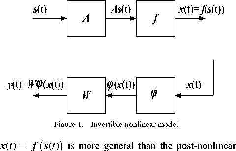
We generalize the MCCA linear BSS algorithm described above to the invertible nonlinear setting depicted in Fig. 1 [4]. This underlying mixing process mixture model proposed in [16] because the nonlinearity f is not restricted to be component wise.

By projecting the input data x ( t ) to some highdimensional feature space via a nonlinear mapping φ and then find the weight matrix W that maximizes the correlation between separate signals. Obviously, if ф = f ¹ and W = A ¹ , then the sources are perfectly recovered and y ( t ) = s ( t ) [3].

The basic idea of kernel-based method allows constructing very powerful nonlinear variants of existing linear scalar product based algorithms by mapping the data x ( t ) ( t = 1,L T ) implicitly into some kernel feature space F through some mapping ф : ^ ^m ^ F . Performing a simple linear algorithm in F , then corresponds to a nonlinear algorithm in input space. All can be done efficiently and never directly but implicitly in F by using the famous kernel trick K j = K ( x , , x j ) = ф р ( x , ), ф ( x j-ф . Kernels offer a great deal of flexibility, as they can be generated from other kernels. In the kernel, the data appears only through entries in the Gram matrix. Therefore, this approach gives a further advantage as the number of tunable parameters and updating time does not depend on the number of attributes being used.

• A. Construct ng reduced kernel feature space

However, a straight forward application of the kernel trick to BSS has so far failed as, after kernelizing, the BSS algorithm has to be applied to a T dimensional problem which is numerically neither stable nor tractable. We need to specify how to handle its possibly high dimensionality. As in Fig. 2, two methods that obtain an orthogonal basis in feature space with reduced dimension are described [3].

A method to obtain the low dimensional subspace is clustering [4]. Denoting the mapped points by px := [ф(x(1)),L , ф(x(T))] and Pv :=[ф(v1),L , ф(vd )] . We assume that the columns of φv constitute a basis of the column space of φx , formally expressed as span(фv) = span(фx) and rank(ф„) = d (16)

And φv being a basis implies that the matrix φvT φv has full rank and its inverse exists, an orthonormal basis can be defined as В := фх (фтфх)-1/2. This basis enables us to parameterize the signals in feature space as real valued d-dimensional signals

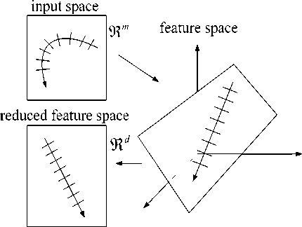
Figure 2. Mapping the input data to reduced feature space.

1 T

So A 1 ,L , A T are the Eigen values of T ф_xф_x with corresponding Eigen vectors φ_xE . Normalizing the first d eigenvectors yields a d -dimensional orthonormal basis

5 : = Ф x E d ( Т Л Г²           (22)

where using ( Т Л ) ^{1 2} to ensure orthonormality and E _d : = [ e 1 ,L , e _d ]. So the input data corresponding in the reduced feature space can be described as

V x ( t ) : = 5 ^T ф ( x ( t )) = ( Т Л ) " ^1/2 Е Т ф Т ф ( x ( t ))

4т

AR

O

^Aa^

M

K ( x (1), x ( t )) M

K ( x ( T ), x ( t ))

V x ⁽ t ) : = 5 ^T Ф ( x ⁽ t )) = ⁽ ф , Ф , ) ' ² Ф ^т Ф ⁽ x ⁽ t )) (17)

By employing the kernel trick

⁽ Ф ^Т Ф v ) ij= Ф ⁽ V ) T Ф ⁽ V j ) = K ⁽ V i , V j )

⁽ Ф ^Т Ф х \_t = Ф ⁽ V ) T Ф ^{( x (} t )) = K ⁽ V ,^{x (} t ))

where i , j = 1,L , d , t = 1,L , T . Substituting (18) into (17) changes it to

V x ⁽ t ) : =

K ( v ₁, v ₁) M

K ( v _d , v ₁)

L

O

L

K ( V 1 , V_d ) 1 " ¹

M

K ^{( V} d , ^V d ) .

K ( v ₁, x ( t )) M

K ( v _d , x ( t ))

Another more direct method to obtain the low dimensional subspace is KPCA (kernel principal component analysis) [4]. For simplicity, we assume that the data is centered in feature space. To perform KPCA we need to find eigenvectors E = [ e 1 ,L , e _T ] and Eigen 1

values X 1 >  L >  A T of the covariance matrix T ф_x ф_x . Now, let Λ be the diagonal matrix with the Eigen values along the diagonal and let

E = ЕЛ

which can also be expressed as

^ T Ф x Ф ^Т ^ ( Ф x^E ) = ( Ф x^E ) ^{Л        (21)}

which are calculated conveniently using the kernel trick.