Nonparametric identification of dynamic systems under normal operation

Introduction. The main objective of identification theory is the model construction based on input and output process variables observations while data about the object is incomplete [1–3]. The article considers dynamic object identification under nonparametric uncertainty [4; 5], when the dynamical model cannot be identified up to parameter vector due to the lack of a priori data. In this case getting transient response and following estimation of an object weight function are reasonable. The basis of this paper is Duhamel integral use, due to the principle of superposition [6; 7]. Identification algorithms of the object in normal operation conditions are described. The research analyses three methods of obtaining weight function estimation using Heaviside function [8; 9], deltashaped input and arbitrary input.

Problem formulation. We assume that an object is a dynamic system described by equation [1], x t = f ( u t , ц t ) where f ( ■ ) - is unknown function; u t - control input variable; ц t - uncontrolled, but measured variable; x t -output variable.

Fig. 1 illustrates a block diagram of the dynamic process [1; 10], with the following notations: x ˆ _t – output of model; u t - control variable; ц _t - uncontrolled, but measured variable; ( t ) – continuous time; t – discrete time; ^ _t , h - random noise influencing the object and output variable measuring channel, with zero mathematical expectation and limited dispersion.

Variables control is carried out at time interval A t . Thus, it is possible to obtain initial input – output variable sample { x i , u i , ц i , i = 1, s }, where s - a sample size.

Non-parametric identification algorithm when standard signals can be input to the object. We could assume that the object is described by a linear differential equation of unknown order. In this case, for zero initial conditions, x(t) is found as where

x ( t ) = X u ( t ) + Х ц ( t ),

t xu (t) = J hu (t -t) u (t) d т ,                (1)

t xц (t) = J hц (t — т)ц(т) dt.

Where h (t -t), h,, (t -t) - weight functions of u И- and ц channels. Weight function is a derivative of the transition function h(t) = k (t).

This problem becomes the weight function estimation, so, first, the transition function needs to be obtained.

As it is mentioned, weight function can be obtained by various means.

First case. We suppose that the object is described by linear differential equation of unknown order. Under zero initial conditions, x ( t ) is found as (1). Transition function is an object reaction to input impact, namely as Heaviside function u ( t ) = 1( t ).

1( t ) =

0, u ( t ) <  0

1, u ( t ) >  0^.

After obtaining transition function, to find its nonparametric estimation is required [11; 12]:

(

k ( t ) = — E k i H |---^L I , sc, i =0        ( c, )

where k_i – transition function estimate, k_i – transition function, t_i – discrete time of measurements, s – sample size, c_s – kernel smoothing, H – kernel function, T – time observation period [2].

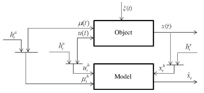
Fig. 1. Identification scheme

Рис. 1. Схема идентификации

We note that kernel function and kernel smoothing satisfy following terms [11; 12]:

1 f t — 1. 1                      1                 f t — t 1

f H|----L | dt = 1, lim    f ф(t)H|----L dt = ф(ti), c         c            s ^0 cc s —ОТ s                           s —ОТ f t — t; 1 „

H - >  0, c >  0, lim sc , ^ от , lim c ^ 0, s        c _t^00 s          s ^OT s

V cs J

where ф ( t i ) - an arbitrary function.

In particular, kernel function would be considered as Sobolev function (5):

0,| t ^— t - l >  c s

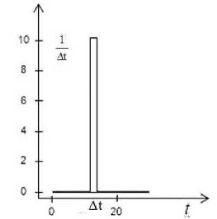
Fig. 2. Delta-shaped function example

H =i

^f —( t — t - ) ² ) 0.827 I_(t_ „,2^2 I^, -----------e ^{V (} t t i ) c s )

I t ^— t - l ^ ^cs .

s

Since weight function h ( t ) is derivative of transition function k ( t ), then

Рис. 2. Пример дельтаобразного входного воздействия

I 1

h(t) = — Zk-H 1---L I, sc, , =0        V c, J

Third case. If control action and object output are known, weight function may be described by (1).

In a discrete form:

where k_i – transition function estimation, k_i – transition function, t_i – discrete time of measurements, s – sample size, c_s – kernel smoothing, H – kernel function, T – time observation period.

Second case. The weight function could be obtained when a delta-shaped function is input, shown in fig. 2. It has got step function type (7), A t - discretization interval

6A(t) = J X,t gat, (7) [At where At, for example, is an equation At = t' — t".

Identification algorithm under normal object operation. Constructing an adaptive object model often requires identification of measuring channels under normal object operation [2; 8; 13]

Therefore, the third case has got the priority in solving the problem of nonparametric identification [4; 6]. The following algorithm when input impact has got sinusoidal type function (as an example) is analyzed below.

I f                                             11

^h- = I x t ^— I Z u - ^At+ Z h 0 1 1 ⁺

V      V - =1          -=1 J J f f11

+ ^xt ^I— Z^/At + Z h , i = 1, s ,

V VJJ

where s - sample size; At - variables control time interval; u_t - control variable; ц _t - uncontrolled, but meas-

ured variable; x_t – object output; h ₀ – value of the

weight function on previous iteration steps.

Therefore, nonparametric process model is:

x s ⁽ t ) =

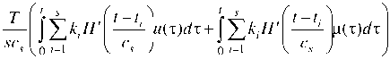
or

■y t s xs (t) =--- [Z huu (t)dt + scs V 0 - =1

s

t _s

fz

0 - =1

where k_i – transition function, h_i – weight function, c_s – kernel smoothing, s – sample size, T – observation period.

Computer experiment. We suggest that dynamical an object is described by a second-order differential equation. It can be represented as:

xt = x“ + xf, xu = 0.25 xu-1 - 0.33 xu-2 + 0.33ut,        (10)

x_t ^f = 0.25 x t- - 0.33 x_t ^f _{- 2} + 0.33u_t .

We could suppose that the equation (10) is used to obtain sampling points. Nonparametric algorithm does not mean the known form of the differential equation, only information on the linearity of an object is known, in contrast with [14; 15]. It should be noted once again that certain equations accepted in this computational experiment remain unknown. Only a priori information about its linearity is known as well as the presence of the principle of a super position. It is important, that taking the transient characteristics for each object channel occurs when the other channel stabilizes [16; 17].

As an arbitrary input signal in the conditions of normal operation of the object, we give a sinusoidal input action u ( t ), it is not a controlling action, but a measured one f ( t ):

u, = sin(0.1 t )

^t                 .                     (11)

f _t = sin(0.05 1 )

Fig. 3 uses following notations: u ( t ) – sinusoidal input action, f ( t ) - uncontrolling, but a measured variable.

We could add a random noise h, that arising in the channel of output signal x(t) measurement h = x k t,                    (12)

where k _t g [ - 1;1], noise level l = 10% .

We calculate a recovery error – w according to the

s

E I x t ^{- x}1 1

W = ^=^         ,                    (13)

E | x t ^- x | i =1

1s where x = V xt - arithmetic mean, x$ (t) - model output. » i =1

Implementing the algorithm (1), we construct a model of the object, shown in fig. 4.

Fig. 4 uses the following notations: x ( t ) – object output; x ˆ( t ) – model output; noise level l = 0%; recovery error w – 0.047, according to the chart and recovery error, this model could be considered as satisfactory.

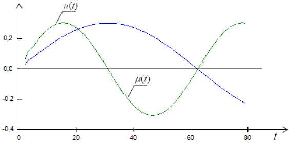
Fig. 3. Arbitrary input actions u and f

Рис. 3. Произвольные входные воздействия u и f

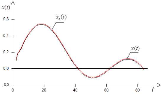
Fig. 4. Object output x ( t ) when the input is an arbitrary sinusoidal signal

Рис. 4. Реакция выхода объекта x ( t ) и модели, при синусоидальном входном воздействии

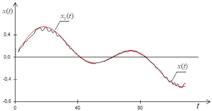
Fig. 5. Object output when the input is an arbitrary sinusoidal signal and noise level 10 %

Рис. 5. Результаты выхода объекта, при синусоидальном входном воздействии при уровне помех равном 10 %

The case when l = 10 % and recovery error w – 0.112 is shown on fig. 5.

Conclusion. The research analyzes the problem of nonparametric identification of linear dynamical objects under the conditions of incomplete data. The main result of this paper is resolution of identification problem in an object normal operation conditions. The paper submits nonparametric linear dynamical system models based on Duhamel integral estimation by means of Nadaraya-Watson statistics.

The main conclusions based on the extensive numerical research of nonparametric models are following: although in practice delta function cannot be submitted to the object input, sometimes it is possible to submit delta-shaped input signal and then construct a satisfactory model. Undoubtedly, noise increase in input-output variables measurement and increase in discreteness of input-output variables control deteriorate an accuracy of nonparametric models.

In addition, it is important to note that a researcher does not know a particular object equation and a differential equation order; moreover, all equations described are analyzed as examples. Therefore, algorithm does not depend on the type of input impact, the main condition is observance of the superposition principle.