Numeric-analytical method for determining the communication equations of Laplace’s transformants of the universal radial unit of externally-pressurized gas bearings

In the study of dynamic quality of externally-pressurized gas bearings is used nonstationary Reynolds’ differential equation [1] which describes the dynamic pressure distribution in the thin gas lubricating gap of loading or throttle unit. Solution of this equation allows to determine the load capacity of the unit and gas flow rate at its inlet and outlet. The main difficulties in the calculation of the dynamics of bearings, relate to obtaining solutions of the equation in view of its nonlinearity.

Within the linear theory, in which integral Laplace transform [2] is applied for research of dynamics of bearings, the solution of the corresponding linearized differential boundary value problems lies approximately as the such problems have no analytical quadratures. Known approximate methods

Taking into account a tendency of complication of the designs using gas-lubricated units and, as a result, complication of the corresponding mathematical models, the search of methods for approximate solutions of noted boundary value problems, which allow to find their decision with a prescribed accuracy is actual. In this regard numerical methods, for which there is no problem of analytical quadratures [5], attract attention. The application of these methods allows to receive the solution of differential problems with an accuracy demanded for practice and possibility of its assessment.

However the circumstance that the structure of linearized and Laplace’s transformed differential equation, includes beforehand unknown Laplace’s variable and some Laplace’s transformants for unit functions, is an obstacle for numerical search of the solution. In this regard numerical and analytical approach to the solution of the specified problems which will allow to find the solution of the boundary value problems deserves attention.

Below it is given a method solving this problem with the example of the universal radial gas-lubricated unit, making radial movements concerning the central equilibrium position.

Mathematical modeling of unit radial movement

The settlement scheme of the unit is shown in Fig. 1.

The unit consists of the cylindrical plug 1 and shaft 2, making movement at which axes of these elements keep a parallel arrangement. These elements are separated by a thin gap of compressed gas under pressure p ( z , φ, t ); gap thickness h (φ, t ) = h 0 – e ( t ) cos (φ), where h 0 – gap thickness at a coaxial arrangement of elements, e – eccentricity of shaft; z , φ – longitudinal and circumferential coordinates, t – current time.

The boundary value problem for function of pressure, which satisfies to Reynolds’s differential equation [1], has the form

Fig. 1. Settlement scheme of radial gas-lubricated unit

1 д r2 дф

,з д p h ³ p

дф

д ( ph ) д t

, p(0,ф, t) = р,(ф, t), p(l,ф, t) = p2 (ф, t), p (z ,0, t) = p (z ,2n, t), — (z ,0, t) = — (z ,2n, t), дф       дф

, p ^{( z} , ф ^,0) = p o ^{( z} ),

where p ₁, p ₂ – functions of gas pressure at inlet and outlet of the unit, p ₀( z ) – gas pressure at a coaxial arrangement of elements, r – the radius of a shaft, l – unit length, μ – viscosity of gas lubricant.

Having taken for scales: p a – environment pressure for pressures; set from the outside h * – thickness of a lubricant gap, r _* – the size and t _* – time scale constants, we will lead a problem (1) to a dimensionless form

\ 4 H³ 'V H³  ' = 2 . ⁵PPH1 ,

R2 дф (   дф J     дZ2       дт

< Р(0,ф,т) = Р(ф,т),Р(L,ф,т) = Р2(ф,т), дР        дР

Р ( Z , 0, т ) = p ( Z , 2 п , т ), д- ( Z , 0, т ) = ^- ( Z , 2 п , т ), дф        дф

. Р ( Z , ф ,0) = - 0( Z ),

where H ( ф , т ) = H ₀ - е ( т ) Cos ( ф ) - the dimensionless thickness of a lubricant gap, e - shaft eccentricity, L = i / r * , r = r / r * - dimensionless length of the unit and shaft radius; Z , т - dimensionless longitudinal

12 µ r ²

coordinate and current dimensionless time; □ = —2-r— - number of squeezing of a gas film [6]. p_ah _* ² t _*

Hereinafter dimensionless sizes are designated by capital letters.

Let’s consider small fluctuations of a shaft concerning its central position. In this case the square of pressure function can be presented in the form

Р ²( Z , ф , т ) = ^ ( Z , ф , т ) = Р 0 ²( Z ) + AY ( Z , т ) Cos ф ,

where AY - a projection function of a deviation from state at a coaxial arrangement of unit elements.

Assuming that eccentricity е = Ae will be small also, after linearization of a problem (2) and applications to it Laplace’s transform, linearized problem for Laplace’s transformants can be written as follows

' d2 AY

< d ² X

I, ав s

- 1 + —— AY = -а $Р Ae,

V Р0 7

AY (0, s ) = AY 1 ( s ), AY ( B , s ) = AY 2 ( s ),

where new variable X = ZIR , B = L/R , а = c R ² / H 3 , в = H ₀ / 2 , s - beforehand unknown variable of Laplace’s transform,

Р 0 ( X ) = Рд [+ Р 20 - Р< ^Х1

– function of lubricant static pressure at a coaxial arrangement of elements, P ₁₀, P ₂₀ – known values of static pressure at unit inlet and outlet.

Boundary functions in (4), as it appears from (3), are related with transformants of pressure deviations by relationships

AY 1 = 2 P₁₀ A P 1 , AY 2 = 2 P ₂₀ A P 2 .

Here line from above marked Laplace’s transformants of the corresponding deviations.

Numeric- analytical method of the solution of a boundary problem (4)

As it is mentioned above, the boundary problem (4) has no analytical decision. It is impossible to apply to it also numerical methods because boundary transformants and Laplace’s variable s aren’t known beforehand. Numeric-analytical method of its solution is given below.

According to the principle of superposition [7] we will find a solution of the problem (4) in the form

AY = T 1 ( Z , s ) AY 1 + T ₂ ( Z , s ) AY 2 + T _E ( Z , s ) A e ,

Having substituted (7) in (4) and having executed separation of functions, we will receive three boundary problems for T -functions:

Г dr-(1+...) t = 0

< d ² X (     P₀ J ¹

dT -( 1 +^a) T = 0. <  d ² X ( P ₀ J ²    '

_ T (0) = 1, T ( в ) = 0,

_ T 2 (0) = 0, T ₂( в ) = 1,

(8)–(10)

dx j d ² X

-

¹ + ^H I T e =-a SP 0 , ^P 0 J

_T e (0) = 0, E T (0) = 0.

Solution of a problem (8)

Having divided the segment [0, B ] into even number of parts n we will execute replacement of a differential problem (8) on finite-differential problem [5]. System of the linear equations concerning values of required function for internal nodal points can be written as

'Tj +. ^{- -} ( a ⁺ b j S ) Ty+ T ,-1 = ⁰,

< T ,0 = 1, T 1n = 0,

⁽ yj = 1,2,..., n — i).

where a = 2 +v², b = ^aev ,v = B — step of finite-differential grid. ^j P ₀( j ν)       n

Having excluded known values of function on the interval ends, we will receive three-diagonal system of the equations

( a + b 1 s )	1	0	...          0	0	0      "	" Th "		"- 1
1	- ( a + b 2 s )	1	...          0	0	0	T ,2		0
... 0	... 0	... 1	...            ... - ( a + b j s )   1	... 0	... 0	... T1.j	=	... 0
... 0	... 0	... 0	...            ... ...            1	... - ( a + b n - 2 s )	... 1	... T 1 , - 2		... 0
0	0	0	...          0	1	- ( a + b n - 1 s ) _	T _ T 1, n - 1 _		. 0

We solve this system by using idea of Cramer’s rule [8].

At first we will find Cramer’s determinant А T 1 _n - 1 . In a matrix of the system (12) its last column we will replace with a column of free members and find determinant of the received matrix, having opened it on the last column. As n is even, we will receive product of number –1 and determinant with the upper triangular matrix, on the main diagonal of which units are located. As such determinant is equal to 1, then А T 1n - 1 = -1. Using a boundary condition T _{1, n} = 0, by means of reverse motion and simple machine-analytical transformations we will find expressions for missing Cramer’s determinants by a recurrent formula, which follows from (11)

А T_u _ , = ( a + bs ) a T_y -A j ( j = n - 1, n - 2,...,1).

As T ₀ = 1 , determinant of a matrix of system (12) is equal to A D ( s ) = A T , ₀( s ).

As an example the solution of the system (12) is found at R = 1.2, L = 1.5, H ₀= 1.2, P ₁₀= 4; P ₂₀= 1; σ = 50; n = 4. The solution of then system is provided by Cramer’s determinants which are polynomials of variable s :

A T 0 =- 5.035 - 9.865s - 4.832s² - 0.654s³,

A T 11 =- 3.400 - 4.106s - 0.938s²,

A T , ₂ =- 2.098 - 1.120s,

A T 13 =- 1,

A T ,4 = 0,

A D = A T₀ = - 5.035 - 9.865s - 4.832s² - 0.654s³.

Thus, values of the T ₁ function in each nodal point represent the relation of polynomials

A T i

Ta^ , ( j = ⁰- n ),

i. e. they are rational functions of variable s . Functions (14) have the identical denominator which is equal to a polynomial of matrix determinant of system (12).

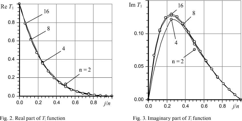
In Fig. 2. and Fig. 3 graphs of the real and imaginary parts of the T ₁( X , s) function at various values n and at constant complex value s = 1- i ( i = V-1) are shown.

The graphs show that the accuracy of calculations accepted for practice is provided at rather small number n of division of the integration interval. So, even at n = 4 error of calculations for graph curves doesn’t exceed 1 %.

Solution of a problem (9)

Differential system of linear equations for the values of T 2 function at the nodal points has the form

^T 2, j + 1    ( a ^{+ b}j s ^{) T} 2, j ^{+ T} 2, j - 1 = ⁰,

T = 0, T n = 1,

⁽ j = 1,2,..., n - 1).

Having excluded known values of function on the interval ends, we will receive three-diagonal system of the equations

- ( a + b 1 s )	1	0	...          0	0	0       "	" T 2 ,1   "		■ 0 "
1	- ( a + b 2 s )	1	...          0	0	0	T 22		0
... 0	... 0	... 1	...            ... - ( a + b j s )   1	... 0	... 0	... T 2, j	=	... 0	.           (16)
... 0	... 0	... 0	...            ... ...            1	... - ( a + bn - 2 s )	... 1	... T 2n - 2		... 0
0	0	0	...          0	1	- ( a + b n - 1 s ) _	_ T 2n - 1 ,		.- 1 .

For this system Cramer’s determinant A T ₂ ,1 = -1. Really, if one opens this determinant on the first column, we’ll receive product of number –1 and determinant with the lower triangular matrix on which main diagonal units are located. Such determinant is equal to unit that proves the statement.

Using a boundary condition T _2,0 = 0, by forward stroke we will find expressions for missing Cramer’s determinants on a recurrent formula, which follows from (15)

A T j = ( a + b j s ) A T j -A j

( j = 1,2,..., n - 2, n - 1).

The system (16) has identical with (12) matrix of the system and its determinant.

The solution of then system for the same as at 3.1 parameters is provided by Cramer’s determinants which also are polynomials of variable s :

A T^ = 0,

A T 21 =- 1,

A T ₂ , ₂ =- 2.098 - 0.698s,

A T ₂ ,3 =- 3.400 - 3.220s - 0.584s²,

A T ₂ , ₄ =- 5.035 - 9.865s - 4.832s² - 0.654s³.

Values of the T ₂ function in nodal points also represent the rational expressions

A T ₂ j    ,

T . =---- -,  ( j = 0... n ).

^{2, 7}     A D

Solution of a problem (10)

By analogy to 3.1 and 3.2 we will write the system of the linear equations concerning values of the T ε function in nodal points

T J ^- ( a + b j S T ' ^TJ1 = ^- C j S,

T = 0, T n = 0,

(j = 1,2,..., n -1), where nj = av2P0(Jv).

Having excluded zero values of function on the interval ends, we will receive three-diagonal system of the equations

( a + b , s )	1	0	...          0	0	0      "	■ T ,1 ■		■ C 1 1
1	- ( a + b 2 s )	1	...          0	0	0	T ,2		c 2
... 0	... 0	... 1	...             ... - ( a + b j s )   1	... 0	... 0	... T j	=- s	... CJ	(20)
... 0	... 0	... 0	...             ... ...            1	... - ( a + b n - 2 s )	... 1	... T n - 2		... Cn - 2
0	0	0	...          0	1	- ( a + b n - 1 s ) _	т , L E , n - 1 J		. c n - 1 .

Now we will find Cramer’s determinant

	c 1	1	0	...          0	0	0
	c 2	- ( a + b 2 s )	1	...          0	0	0
A T ,=- s	... c j	... 0	... 1	...             ... - ( a + b j s )   1	... 0	... 0	.                       (21)
	... cn - 2	... 0	... 0	...             ... ...            1	... - ( a + b n - 2 s )	... 1
	cn - 1	0	0	...          0	1	- ( a + b n - 1 s )

Having opened (21) on the first column, we will find out that minors of the received sum are equals to opposite on a sign Cramer‘s determinants of the system (12). On this basis n-1

A T ,1 = s Z C j A T , .

j = 1

Using a boundary condition T _{ε ,0} = 0, by a forward stroke we will find expressions for missing

Cramer‘s determinants on a recurrent formula, which follows from (19)

^A T _E , j ₊ 1 = ( a +     ) ^A T _E , j -^A T _E , j - 1

_( j = 1,2,..., n - 3, n - 2).

- C j S A D ,

At numeric-analytical definition of polynomials (22) their members at j >  n are equal to zero, therefore they can be dropped.

For the same as at 3.1 and 3.2 values of parameters corresponding Cramer’s determinants are equal to

A T _E 0 = 0,

^{A T} e ,1 =

A T . 2 =

- 82.176 s - 11.483s² - 0.0855s³,

- 100.676 s - 67.373s² - 9.270s³,

A T _E , ₃ = - 69.280 s - 36.829s² - 5.180s³, A T _E^ = 0.

Values of T ε function in nodal points are determined by a formula

A T ,

T ,=        ,  ( j = 0... n ).

ε , j D ,

Transformant of unit load capacity deviation

Load capacity of the unit is defined by a formula [1]

2π                 l w = r j cos^)dфJ(p-pa)dz.

Having taken for scale of forces complex f * = n r . ² p a according to (3), (6), (7) we will receive a formula for Laplace’s transformant of dimensionless load capacity deviation of the unit

A W = — B ^{AY (} X , s ) dX = W A P 1 + W ₂ A P 2 + W_E A e ,

2 ^J P 0 (X )          ^{1         2          E}

where

W = P_1OR² B T 1 dX , W = P₀R² B T 2 dX , W = R 2 B T E dX . 1      10                    2      20                      ε

₀ P ₀₀ P ₀2 ₀ P ₀

As T -functions are rational functions and they have common polynomial Δ D ( s ) of their denominators, having applied to their numerators Simpson’s rule [9] for numerical integration of grid functions, we will find first Laplace’s transformant dynamic equation of the unit

A D ( s ) A W + A W ( s ) A P 1 + A W ₂( s ) A P 2 + A W _E ( s ) A e = 0,

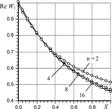
Fig. 4. Real part of W 1 function, s = X (1– i )

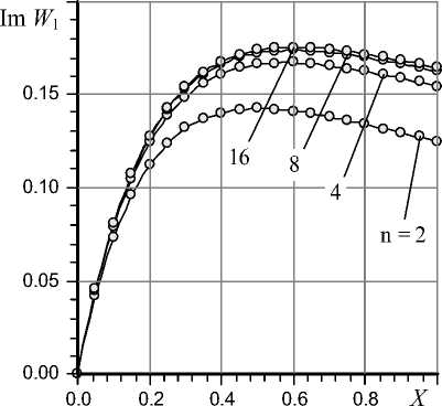
Fig. 5. Imaginary part of W 1 function, s = X (1– i )

where A W 1 , A W₂, A W _E - the polynomials of variable 5 received by elementary transformations at numeric-analytical integration of Cramer’s determinants of (13), (15), (22) on Simpson’s rule calculation process.

In that case for the examples of calculations, given above, polynomials are received

^A W ( ⁵ ) = ^5.051 + ^{4.757 5} + L368S² + 0.098s³,

^A W 2 ^{( 5} ) = ².⁰⁷9 + ².⁴³8 ⁵ +       . + ⁰.09^8s 3 ,

A W _E ( 5 ) = 21.760 5 + 14.6876s² + 2.335s³.

Local transfer functions (25) are clearly equal to

W =A W 1, w =A W 1 W =A W .

• ¹   A D   ² A D   ^E    A D

Submission about impact of number n on the accuracy of carrying capacity transformant for different values of variable s give graphs in Fig. 4 and Fig. 5.

From these graphs it is visible that sufficient accuracy for practical calculations is provided at n = 4.

Transformant of longitudinal deviation of local flow rates on inlet and outlet of unit

The mass flow rate in the direction of longitudinal coordinate on a chord r Aф of the small length, given to its angle, is defined by a formula [1]

Лш q =

r

12 ц^ T Aф

Ф j +

3 d p hpd ϕ ,

^J A„      ^d z

• ^ш j - T

where M ,T, ц - universal gas constant, absolute temperature of gas and its viscosity.

Assuming that temperature and viscosity as constants and having taken for the scale of mass flow h3p2

rates a complex q * =---—, we will receive a formula for defining the corresponding dimensionless

6цЭТТ mass flow rate in any cross section of the unit

Q = - RH³ P . a z

Taking into account (3), (5), (6) after linearization of formula (28) Laplace’s transformant of flow rate deviation can be written as

A Q ( X , 5 )

In V , ы 3 d AV 1 - D_n „Ae + H« ---- .

I Q 0        0 dX I

where d q о = 3 H 2 ( P - P 0 ) / B .

Transformant of a local flow rate deviation at a unit inlet

For definition of this transformant we will use the relation (7). We will find derivative of function

AV using initial unilateral trinomial formulas for Cramer’s determinants of the corresponding grid T -functions [5]

_> = d A T j (0,5 )

^{1, j}        dX

-^A T j2 + ^{4 A} j - ^{3 A} j

2 ν

( j = 1,2, e ).

Formulas (30) provide the second order of accuracy concerning a grid step v .

Using (29), (30) we will receive a second communication formula of unit model for transformant of input flow rate deviation A Q ₁ ( 5 ) with corresponding transformants of eccentricity and both pressures at inlet and outlet of unit

A D ( 5 ) A Q 1 + A Q 1,1 ( 5 ) A P 1 + A Q _u ( 5 ) A P 2 + A Q 1 , ( 5 ) Ae = 0,                                   (31)

where A Q 1,1 ( 5 ) = 2 P_№ H 3№_и , A Q _L2( 5 ) = 2 P₂ o H 3 A D 1,2 , A Q _L e ( 5 ) = D q 0 A D + H o3 AD_Tf .

For the above examples we obtain polynomials

A Q 11 ( 5 ) = 79.65 + 316.1 5 + 237.6s² + 43.42s³,

A Q₁₂ ( 5 ) = - 10.52 + 3.857 5 ,

A Q_{1 e} ( 5 ) = - 261.0 + 1141.8 5 - 857.9s² - 156.0s³.

The submission of influence of number n on accuracy of calculation of a transformant of input local flow rate at various values of Laplace’s variable s is given by graphs in Fig. 6 and Fig. 7.

The graphs show that to ensure acceptable accuracy of the real part of Q ₁ function n = 4 is enough, the imaginary part in this case requires n > 4.

Transformant of a local flow rate deviation on a unit outlet

We will define derivative of function (29) using end unilateral trinomial formulas for Cramer’s determinants of the corresponding grid T -functions [5]

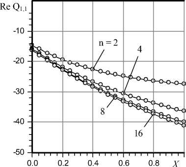
Fig. 6. Real part of Q 1,1 function, s = X (1– i )

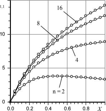
Fig. 7. Imaginary part of Q 1,1 function, s = X (1– i )

K D 2,j =

d ^A TA ^B,s ) dX

^{3 A} j ^- 4 ^A j - I +A j - 2

2 ν

( j = 1,2, e ).

Formulas (32) also have the second order of accuracy.

As a result we will receive a third communication formula of unit model for transformant of an output flow rate deviation A Q ₂( s ) with corresponding transformants of the unit

^{A D (} s ) ^{A Q} 2 =^{A Q} 2,1 ⁽ s ^{) A P 1 +A Q} 2,2 ⁽ s ^{) A P 2} + [ D Q 0 ^{+A Q} 2, e ⁽ s ) ] ^Ae , where A Q 21 ( s ) = - 2 PH 3 A D 2 j , A Q 22 ( s ) = - 2 PH 3 A D 22 , A Q 2 ₆ ( s ) = - H 3 A D 2 ₆ . ,       ,,        ,,      ,

For the examples given above polynomials are received

A Q ₂₂( s ) = 42.07 - 24.78 s ,

A Q ₂ , ₂( s ) = - 19.91 - 96.29 s - 67.24s² - 10.86s³,

^{A Q} 2,⁽ s ) = ^{- 261}.0 ^{- 23}.59 s ^- Ms^{2 -} 2.²⁶¹s³.

Submission of influence of number n on accuracy of calculation of a transformant of output local flow rate at various values of Laplace’s variable s is given in Fig. 8 and Fig. 9.

For the given values of parameters sufficient accuracy for practice is provided at n = 4–8.

Conclusion

The equations (26), (31), (32) allow to establish relations of integro-differential Laplace’s transformants of carrying capacity A W ( s ) and local mass flow rates A Q ₁( s ), A Q ₂( s ) at inlet and outlet of the unit with transformants Ae ( s ), A P 1 ( s ), A P ₂( s ) of eccentricity and pressures at inlet and outlet of unit. Required accuracy of the calculation of T -functions can be provided by selecting the number n of partitions of integration interval.

These equations give ready formulas for calculating the dynamic criteria containing such units of radial one-row, multi-row ordinary passive or active (with zero or negative compliance of carrier gas films [10]) externally pressurized and other gas bearings, in which radial movement of their movable elements is made.

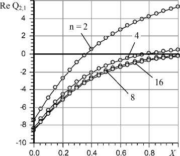
Fig. 8. Real part of Q 2,1 function, s = X (1– i )

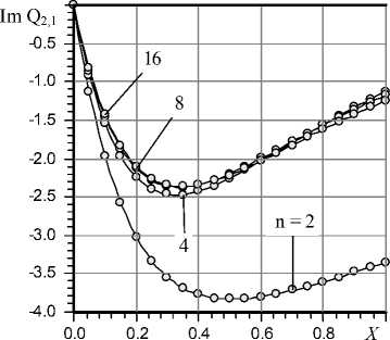
Fig. 9. Imaginary part of Q 2,1 function, s = X (1– i )