Numerical simulation for direct shear test of joint in rock mass

Published Online November 2010 in MECS

Joints exist widely in rock mass, and its characteristic has great influence on the failure characteristic of rock mass[1-3]. So it is among the most important factors in understanding and estimating the mechanical behavior of a rock mass. The shear behavior of joint is combination of complicated phenomena, such as normal dilation, asperity failure and contact area [4,5]. Considerable efforts have been devoted to explaining the shear strength and behavior of joint over the last four decades [6-9]. The difference of the strength, deformation characteristic of joint will lead to the different strength and deformation of rock mass. The direct shear test (DST) is very popular to test the strength of joint owing to its simplicity [10-12]. The conventional direct shear test apparatus [13,14], as shown in Figure 1, has both an upper and a lower shear boxes, and the sample is sheared along the plane between them by pushing the upper shear box horizontally with a normal (vertical) load applied to it. The shear force is measured with a bearing ring or a load cell that is attached to the upper shear box. A frictional force is generated at the attachment point when the upper shear box tends to move up/downward due to the volume change of the sheared sample (dilation or contraction). Sometimes, to prevent the titling of the upper shear box during the shearing process, a clasp is set on the opposite of the attachment point. The frictional force at the attachment point and the clasp restrain the up/downward movement of the upper shear box. Consequently, the frictional force between the interface of the upper shear box and the sample is generated due to the volume change of the sheared sample. Owing to the influence of this interface friction, the applied normal stress is generally lower for dilative specimens (like coarse granular soils) but higher for contractive ones than the true values on the shear plane.

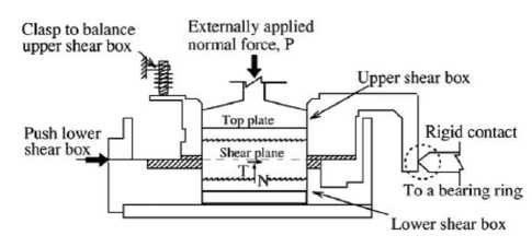
Figure 1. Schematic of conventional direct shear test device [14]

Project number: Forefront Research Program of Central South University (2010QZZD001).

Many scholars have done much work on the mechanical characteristic of joint. In the past, the studies are mainly done with the laboratory test and the theoretical analysis, but the laboratory tests need some cost, and the theoretical analysis has its limitation due to some assumption are needed in applying. So we want to find some more methods to study the topic, fortunately, in recent years, rapid advances in computer technology and sustained development have pushed the numerical analysis methods like the fast lagrangian analysis of continua three dimensions (FLAC3D) to the forefront of geotechnical practice [15-18]. In the present paper, the direct tests of joint are done to study the strength and deformation of joint, which will give some guidance for the real practice and the analytical studies.

• II.    N UMERICAL SIMULATION FOR JOINT

Joint is modeled with the interfaces element [19] in FLAC3D, which is represented as collections of triangular elements (interface elements), each of which is defined by three nodes (interface nodes). Interface elements can be created at any location in space. Generally, interface elements are attached to a zone surface face; two triangular interface elements are defined for every quadrilateral zone face. Interface nodes are then created automatically at every interface element vertex. When another grid surface comes into contact with an interface element, the contact is detected at the interface node, and is characterized by normal and shear stiffness, and sliding properties. Each interface element distributes its area to its nodes in a weighted fashion. The entire interface is thus divided into active interface nodes representing the total area of the interface. Figure 2 illustrates the relation between interface elements and interface nodes, and the representative area associated with an individual node.

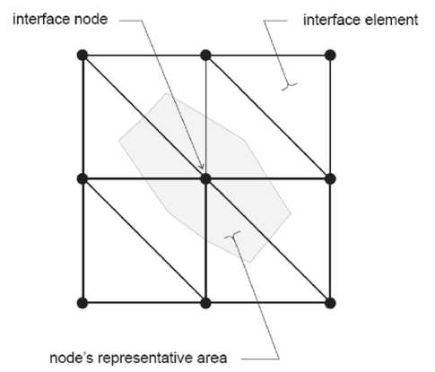
Figure 2. Distribution of representative areas to interface nodes

During each time step, the absolute normal penetration and the relative shear velocity are calculated for each interface node and its contacting target face. Both of these values are then used by the interface constitutive model to calculate a normal force and a shear-force vector. The constitutive model is defined by a linear

Mohr-Coulomb shear-strength criterion that limits the shear force acting at an interface node, stiffness, bond strengths, and a dilation angle that causes an increase in effective normal force on the target face after the shearstrength limit is reached.

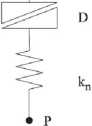
The normal and shear forces that describe the elastic interface response are determined at calculation time ( t + Δ t ) using the following relations, shown in Figure 3.

F t ⁺¹ t ) = k . u , A + » . A (1)

F , "¹¹ t ) = F ) + k , &  u Si *“ /2) A + »„ A (2) where F n ⁽ t ⁺¹ t ) is the normal force at time ( t +A t ); F si ⁽ t ⁺¹ t ) is the shear force vector at time ( t +A t ); U n is the absolute normal penetration of the interface node into the target face; 1 U i is the incremental relative shear displacement vector; O"n is the additional normal stress added due to interface stress initialization; k_n is the normal stiffness; k , is the shear stiffness; CT _si is the additional shear stress vector due to interface stress initialization; A is the representative area associated with the interface node.

target face

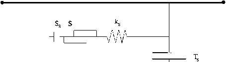
S = slider Ts = tensile strength Ss = shear strength D = dilation ks = shear stiffness kn = normal stiffness

• Figure 3. The mechanical characteristic of node in interface

  III. M ODELING

  

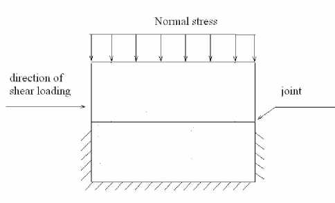
  Figure 4. Direct shear test model

  
  

Direct shear test model shown in Figure 4, then according to this model, the numerical calculation model is founded by FLAC3D, as shown in Figure 5.

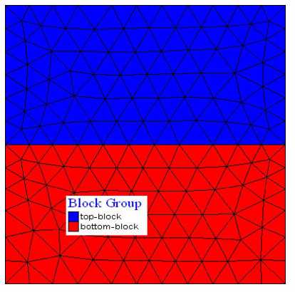
(a) two dimensional view

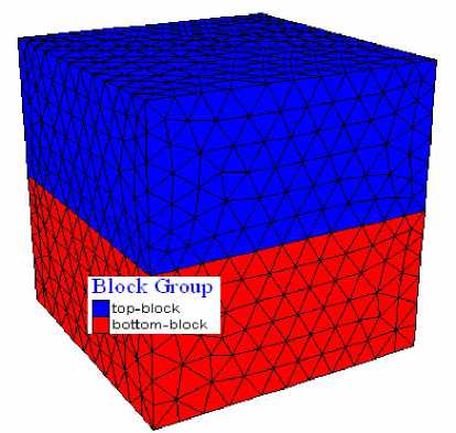
(b) three dimensional view

Figure 5. The numerical model

The numerical model is divided to two groups, topblock and the bottom-block. Size of each block are the same with 250mm x 230mm x 120mm. The shear loading velocity is set to be 1 x 10-3mm/step, where step is the calculation step in FLAC3D. Interfaces have the properties of friction, cohesion, dilation, normal and shear stiffness, tensile and shear bond strength. It is recommended by FLAC3D that the lowest stiffness consistent with small interface deformation be used. A good rule-of-thumb is that kn and ks be set to ten times the equivalent stiffness of the stiffest neighboring zone. The apparent stiffness (expressed in stress per-distance units) of a zone in the normal direction is, max

4K + 4 G

Nz ■ min

where K &  G are the bulk and shear modulus, respectively; and A z _min is the smallest width of an adjoining zone in the normal direction — see Figure 6.

The max [ ] notation indicates that the maximum value over all zones adjacent to the interface is to be used.

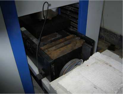
(b) direct shear test device

Figure 7. The direct shear test specimen

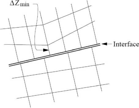
Figure 6. Zone dimension used in stiffness calculation

(a) rock joint sample

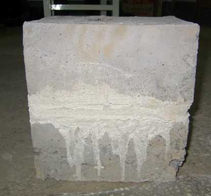
The whole model is fixed in three directions on the bottom, and horizontal direction on each side. Linear Mohr-Coulomb criterion is taken to describe the failure behavior of rock mass. Parameters of the rock are set to be, 2.0GPa for elastic modulus, 23.0kN/m3 for unit weight, 0.20 for poisson’s ratio, 0.3 MPa for cohesion, 37° for friction angle, 10° for dilation angle, and 0.4MPa for tensile strength. The parameters for joint are set to be, 10.0kPa for cohesion, 28.0° for friction angle, 6° for dilation angle. The normal stress are set to be 3.5MPa, 5.0MPa, 6.5MPa, 8.0MPa and 9.0MPa according to the normal stress applied in the laboratory test. The sample and direct shear device used in laboratory test are shown in Figure 7.

• IV. R ESULTS AND DISCUSSION

• A.    Stress distribution of the joint

Figure 8 shows the shear stress distribution on joint, indicating that, the shear stress increases gradually until the maximum value from the left to the right, which is the loading direction. The contour of the maximum shear stress shows the shape of saw tooth in a very small area. And with the increase of the normal stress, the distribution area of the maximum shear stress does not change much, indicating that, the magnitude of the normal stress has little affect on the distribution of the shear stress. When the normal displacement velocity is smaller than some certain magnitude, the distribution of the normal stress on joint shows the similar discipline of the shear stress, shown in Figure 9.

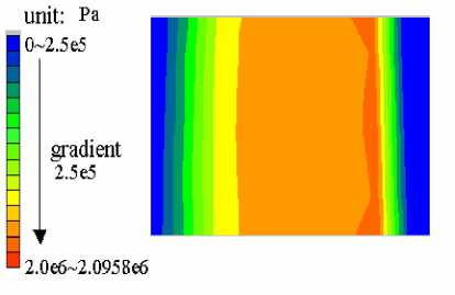
Figure 8. The shear stress contour when the normal stress on the sample equals to 5Mpa

• B.    Deformation characteristic of the joint

2.0

Figure 10 shows the relationship between shear stress and shear displacement when the normal stress on the rock samples is 5 MPa. From the figure, we can see that, during the initial phase of shear moving, the shear displacement increases slowly with the increase of shear stress. The deformation of the joint shows the elastic characteristic. And we can get the shear stiffness of joint by dividing shear stress with shear displacement, the shear stiffness of joint reduces during the shear loading procedure. When the shear stress reaches its peak value, the shear displacement will become larger and larger while the shear stress almost remains the same, indicating the failure of the joint. When shear displacement is small, the shear stress increases linear with the shear displacement. But when shear stress increases larger enough to conquer the friction stress, the relationship between the shear stress and shear displacement shows the nonlinear characteristic. And the result from the laboratory test is obtained to compared to that from numerical modeling, shown in Figure 10, indicating that, the results from both methods can meet well with each other, then the numerical modeling is validated, except that, the shear strength from the laboratory is a little smaller than that from the numerical calculation, due to reason that, the real specimen has more joint and some crannies in the rock body to weaken its strength.

1.5

numerical modeling

laboratory test normal stress σ =5.0MPa

-2    0     2     4     6     8    10    12    14    16    18    20

Shear displacement /mm

-0.5

Figure 10. The relationship between shear stress and shear displacement of the joint

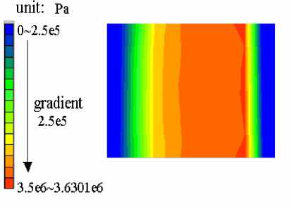
Figure 9. The normal stress distribution of joint when the normal stress on the sample equals to 5Mpa

Figure 11 shows the relationship between the normal displacement un and shear displacement us of joint when the normal stress on the rock sample is 5 MPa. The normal displacement of joint increases in the linear form with the increase of shear displacement of joint, whose relationship can be fitted by the following equation, un = a + b • us (4) where, a is the normal displacement of joint during the shear loading; b is the slope of curve of the relationship between shear displacement and normal displacement.

By fitting, we can obtain the parameters for a =-0.13277, b =0.10392, the fitting coefficient is R =0.99985,

indicating that, if there is no shear displacement, the normal displacement is minus due to the normal stress on the sample. And if the shear loading is placed, the top block of sample is moved to make the normal displacement become larger and larger. So it can be concluded that, the parameter a is larger with larger normal stress unless joint is compressed to failure.

effect, when the shear failure of the joint occurs, the dilation will happen in the rock samples. If the normal stress is large, the dilation will be controlled, and high magnitude of the dilation stress will be produced to lead to the reduction of the effective normal stress and the shear strength of the joint. So, if the normal stress is small, even under some certain value, the shear failure will not happen in the joint.

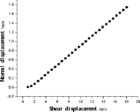
Figure 11. The relationship between the normal displacement and shear displacement

Shear displacement /mm

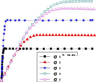
Figure 13. The relationship between the shear stress and shear displacement with different the normal stress under the laboratory test

C. Strength characteristic of joint

3.5MPa

5.0MPa

6.0MPa

9.0MPa

8.0MPa

-1      0      1      2      3      4      5      6      7      8

Shear displacement/mm

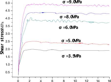
From Figure 12 and Figure 13, both the results from the numerical modeling and laboratory tests indicates that, with increase of the normal stress, the peak value of the shear strength will increase, which is caused by that, joint is compressed densely under the normal stress, and cause larger shear stress to make the shear failure of the rock mass. The relationship between the shear strength τ _s and normal stress σ shows the linear characteristic with the increase of the normal stress (2MPa~5.5MPa, in Figure 14), which is in the accordance the Mohr-Coulomb criterion. According to the Mohr-Coulomb failure criterion, the relationship of τ _s and σ can be fitted as, τ _s = c + σ _n ⋅ tan φ           (5)

where, c and φ are the cohesion and friction angle of joint.

Figure 12. The relationship between the shear stress and shear displacement with different the normal stress under the numerical modeling

During the direct shear test with the combination of the normal stress and shear stress, the joint will occur slipping failure if the shear stress on the joint is larger than shear resistance capacity of joint. When joint slipping occurs, the relationship between shear stress and shear displacement is the linear for the initial phase. But when the slipping rock sample keeps moving, the relationship between the shear stress and shear displacement becomes nonlinear to lead to the shear stress reaching its peak value. And because of the dilation

TABLE I.

F ITTING RESULTS FOR THE LABORATORY TEST AND NUMERICAL

CALCULATION

Case	Fitting parameters c /MPa       φ / °		Coefficient R
Laboratory test	0.01113	28.69	0.98344
Numerical calculation	0.06267	30.12	0.99998

By fitting for the data from the numerical calculation and laboratory test, the results are shown in Table I, showing that the results from the numerical modeling are a little larger than that from the laboratory test, but the differences are small, indicating the results from the numerical modeling is correct.

fitting the data of shear loading velocity and shear strength of joint with the equation,

Ts = m + n • v

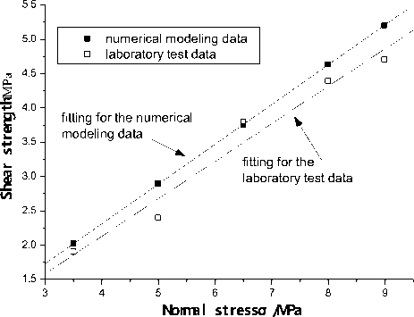
Figure 14. The relationship between the normal stress and shear strength

D. Effect of shear loading velocity to the shear strength of joint

Normal stress σ=3.5MPa

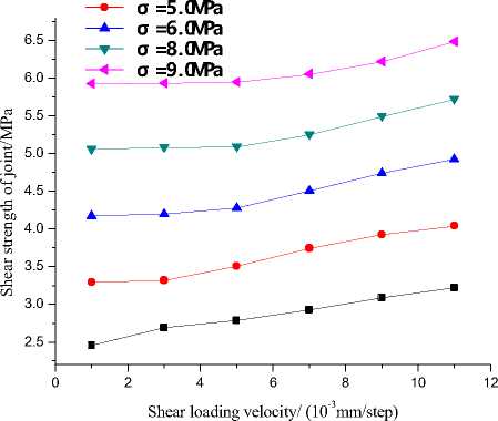
Figure 15. Effect of the loading velocity to the shear strength of structure plane

In order to study the effect of shear loading velocity to the shear strength of joint, the shear loading velocity is changed in the range of [1,11]×10-3 mm/step, then the corresponding shear strengths of joint are recorded, as shown in Figure 15. With increase of shear loading velocity, the shear strength Ts of joint will increase gradually. But with the increase of normal stress, the slope of the curves become smaller, indicating that, the increase of normal stress will decrease the effect of shear loading velocity to the shear strength of joint. Besides, by where, m and n are the fitting parameters.

The fitting results are shown in Table II, indicating that, with increase of normal stress, the fitting coefficient become smaller, the relationship between shear loading velocity and shear strength of joint change from linear form to nonlinear form.

TABLE II.

F ITTING FOR THE EFFECT OF LOADING VELOCITY TO THE SHEAR STRENGTH OF STRUCTURE PLANE

Normal stress Q n /MPa	Fitting equation	Fitting parameters		Coefficient R
		m	n
3.5		2.41938	0.07387	0.99462
5.0		3.14166	0.08292	0.98505
6.5	t = m + n • v	3.99104	0.08013	0.96796
8.0		4.87711	0.06767	0.93175
9.0		5.77210	0.05355	0.90885

V. C ONCLUSIONS

• (1)    The direct shear test of the joint in the rock mass is well simulated by the numerical method, while the joint is simulated by the interface element.

• (2)    The relationship between the shear stress and normal stress shows the linear characteristic with the increase of the normal stress, which is in the accordance with the Mohr-Coulomb criterion. The shear stress increases gradually until the maximum value from the left to the right, which is the loading direction.

• (3)    The stress distribution of the joint, deformation characteristic of the joint, and strength characteristic of joint are analyzed to give some guidance for the real situation and the analytical studies. The result from the numerical modeling method is close to that from the laboratory test, which confirms the validity of the numerical method.

A CKNOWLEDGMENT

This work was financially supported by the Forefront Research Program of Central South University (2010QZZD001).