Numerical simulation methods of electromagnetic field in higher education: didactic application with graphical interface for FDTD method

Published Online August 2018 in MECS DOI: 10.5815/ijmecs.2018.08.01

The computer-assisted training is a modality of students’ individual education using computer software that guides step-by-step the student’s path to knowledge by his or her own effort and pace of understanding [1,2,3]. In the modern teaching, it is successfully used the illustration of various aspects using computer-aided applications with graphical interface that are instructional activation methods treated by the general didactics as distinct methods [4,5,6,7,8]. When teaching the numerical methods for the determination of the electromagnetic field, the computer-aided application with graphical interface enables the interactive access to the theory of the method, the design and implementation of the basic algorithm into a programming language accessible to the students, the design and implementation of certain material propagation environments, implementation of some source models and, last but not least, the visual simulation in time and space of the propagation phenomenon whose evolution is hardly accessible to direct observation.

For example, as numerical method used for the electromagnetic field determination, we chose the finite-difference     time-domain     method     (FDTD)

• [9,10,11,12,13,14,15]    used in the analysis of electromagnetic field interaction with the matter, and the implementation of the computer-aided application with graphical interface was made using the GUIDE Matlab tool [16,17,18,19,20,21]. The FDTD method is based on solving the Maxwell's equations in differential form. Basically, the method consists of replacing the differential equations with finite difference equations [9], [13,14]. The best known implementation of FDTD is the Yee algorithm [9], [13,14], in which the space is discretised into a cubic grid, in whose nodes the environmental  properties and  the value of  the

8.85 - 10^-12 [F/m]) and Ц 0 is the air permeability ( ц ₀ = 1.256 - 10 -6 [H/m]).

electric/magnetic field are memorised. The spatial and temporal derivatives are replaced by central differences. To update the electromagnetic field at each point in space, we use a leap-frog algorithm (interleaving in time of the E and H components). The excitation applied at the initial time is known, and the time evolution of the electromagnetic field is going to be calculated [9], [13,14].

In an FDTD analysis of the electromagnetic field, the following aspects should be considered in particular [9], [13,14]: accuracy of results, numerical dispersion and algorithm stability. A method is considered to be accurate if the numerical solution is very close to the exact solution. Generally, there are 3 types of errors that affect the accuracy of a result: modelling errors, discretisation errors, and rounding errors. The numerical dispersion is caused by space discretisation. The discretisation leads to the emergence of new spectral components that propagate at different speeds. A numerical solution is stable if it produces a bounded result for a limited input variance. The numerical accuracy, dispersion and stability are influenced by spatial and temporal sampling resolutions. The spatial resolution must be less than         ( λ is

.     min min the minimum wavelength propagating in the analysed field). The temporal resolution is selected later, ensuring the numerical stability of the algorithm. The memory requirements for FDTD are proportional to the number of cells in the computing domain.

In this article we present a didactic application with graphical interface, programmed using the Guide Matlab to simulate the electromagnetic waves propagation through various environments and applying the finite-difference time-domain method (FDTD). The FDTD method is based on solving the Maxwell's equations in differential form.

For linear, isotropic and non-dispersive environments [9], [13,14]:

——       ——

D = eE

——        ——

B = pH

• II.    Solving Maxwell's Equations Using the Finite-Difference Time-Domain Method (FDTD)

The term J may contain components that act as independent sources for the fields E and H (hereinafter,

A. Maxwell's equations

they will be denoted by J    ). Therefore:

We consider a space region in which the material environment can absorb electrical or magnetic energy. The Maxwell's equations [9], [13,14] in differential form are:

——     ——               ——

J = J source + O E

By replacing (8), (9) and (10) in (1) and (2), we obtain:

д B д t

——

-VxE

a H a t

- 1 v xE— в

(the law of electromagnetic induction)

——

— = V xH - J д t

д E д t

= 1 VXH - 1 (Jsource + oE) e      e

(the law of magnetic circuit)

The equations (11) and (12) are rewritten using the projections on the coordinate axes:

—

VD = Pv

(the law of electric flow)

—

VB = 0

(the law of magnetic flow)

In eqs. (1)-(4), E is the electric field intensity [V/m], H is the magnetic field intensity [A/m], D is the electric induction [C/m²], B is the magnetic induction [Wb/m²], J is the electric current density [A/m²] and p v is the charge density [C/m³].

Material laws [9], [13,14]:

—— J = oE (5) D = E0 e+p (6) B = p0 (h+Mi) (7) ди^ = 1 дEy  д д t   p дz   дy

д H y	1	" д E z	д E x "  —
д t	в	_ д x	д z _	(14)
д H z	1	" дE x	д Ey" —
д t	p	_ay	д x J	(15)

дEx д t =1 e "дН^ _ дy дHy дz sourcex + OEx ) (16) дEy дt 1 e "дН, L дz _ дН^ дx sourcey + °Ey ) (17) дEz д t =1 e "дHy L дx _ дН^. дy sourcez + OEz ) (18) where: a is the electrical conductivity of the environment [S/m], P is the electrical polarisation of the environment, M is the magnetisation, s0 is the air permittivity (s0 =

The equations (13) and (18) are the basis of FDTD numerical algorithm for describing the interactions between the electromagnetic waves and the environments in question.

B. Maxwell's equations with finite differences

u

( i A x, j A y,k A z )

not n i, j,k

Given a function of the form u = u(x, t) , dependent on time, t, and space, x, according to a certain law. In a numerical simulation, the solution of an equation can only be an approximation of the analytical solution because of the discretisation inherent to any calculation carried out with a numerical system. Therefore, if u(x,t) is the solution of an equation, this one can be determined only in discrete points having the form (xi,tn) , where i = spatial index, n = temporal index. In case of expansion in Taylor series of the function u(x, t) around the point x i , for a given moment, tn , we obtain [9], [13,14]:

where: A t = temporal increment, assumed to be uniform within the observation interval; n = integer number; A x, A y, A z = space increments on the three directions of the coordinate system; i, j, k = integer numbers.

Thus, if we consider the derivative of u with respect to x , evaluated at the moment tn = n A t , it will be written as follows, using the equations with finite differences:

u(Xj - A x)L = u L, - A x — L, +

' i           t n        ^x i -t n         у x ^xl -t n

nn d —                          —i+1/2,jJk   — - 1/2,j,k

— ( i A x, j A y, k A z, n A t ) =-- +

5 x                        A x

+ OA y,(Ay)2,(A-y,(at)2 ]

( A x ) ²  d ²— .        ( A x ) 3  d 3 — .

⁺ 2  d x ⁷^     6"" 'Ix ^ ' x i t n

+ ...

• —(x, + A x) L = — 1.,  + A x — L +

v i          t n       xit n        d x x i -t n

( A x ) ² d 2 — .        ( A x ) ³ d 3 — .

• ⁺ 2   d x ⁷ ^ ⁺ 6  'lx 3 ' ^{xi,,n +} ’

The increment of ± 1/2 at the index i (on the x-axis) denotes a spatial difference of ± ^ ■ A x . Yee chose this notation to insert the components E and H into the space at intervals of ^{A x} /2. Similarly, we write the partial derivatives of u with respect to y and z. The derivative of u with respect to time, evaluated at a given point in space, (i, j, k), is:

If the two relations are subtracted, an approximation is

obtained for

d—

8x

n + 1/2   n -- - 1/2

d —                           ^—i,j k   ^{- —}i,j k ,

— (iAx, jAy, kAz, nAt) = —----------+

8 1                          A t

+ O [(Ax у'.Ay) )2 ,(Az )■'-An)-2 ]

d —   — (x + Ax )tn -—(xi- A )tn

d x

2 A x

+ O A )2 ]

Using the above notations, the Maxwell’s equations with finite differences are written as follows [9], [13,14]:

By summing the two equations and dividing by ( A x У ,

8 2— an approximation for      is obtained as follows:

d x

^{n +} 1^{/2               n} - ^1/2

E x ij + 1/2,k + 1/2   E x Vj + 1/2,k + 1/2 _

A t

^e i,j + 1/2,k + 1/2

, H z i j+ 1/2,k + 1/2   H z i -j ,k + 1/2

A y

—

nn

Hy ij + 1/2,k+1 Hy i;y+1/2,k _ , sourcex

i -j+ 1/2,k + 1/2

d 2— dx2

^{— ( x} i + ^A ) t_n ^{- 2—} x , y „ ^{+ — (} x ^{- A} ) t_n ( A x)

+ O [(Ax)2 ]

^a i,j + 1/2,k + 1/2 ■ E x i;j + 1/2,k + 1/2 )

where O [ ( A x У ] = 2^nd

order error, occurred because the

terms of the Taylor series whose order is higher than 2 have been neglected.

The algorithm is not time-dissipative, meaning the numeric waves that propagate across the grid are not mitigated over time due to the applied numerical method.

A point in the discretised space, whose coordinates are (i, j, k), will be associated with the quantity ( i A x, j A y, k A z ) . A function dependent on time

and space will be written as follows:

By the equation (26), we wanted to evaluate the Ex component of the electric field at time n , in the point whose coordinates are (i, j+1/2, k+1/2). It can be seen that all the values of the field components in the right side of the equation are evaluated at time n , including the value of the electric field Ex produced due to the conductivity a of the material. Since the values of Ex at time n are not stored in the memory, but only the values of Ex at time n-1/2, it is necessary to estimate these values. A method used to estimate Ex at time n is the so-called semi-implicit approximation (arithmetic mean):

E x \ i,j + 1/2,k + 1/2

n + 1/2

E x \i,j + 1/2,k + 1/2

—

^{n — 1/2}

E x ij + 1/2,k + 1/2

(

1 —

n ^{+ 1/2}      _

E x i,j + 1/2,k + 1/2 =

" i,j + 1 /2,k + 1/2 ' ^A t 2 ^£ i, j + 1 / 2,k + 1/2

It is assumed that the values of Ex are stored in the memory at time n-1/2, but not at time n+1/2. After substituting (27) into (26) and rearranging the terms, it results:

к

1 + " i,j ⁺ 1 ^{/2k + 1/2} • ^At 2 ^£ i,j + 1/2k + 1/2  ₇

•F I n ^{— 1/2}       +

E x i,j + 1/2,k + 1/2 ⁺

A t

к

^£ i,j + 1 / 2,k + 1/2

(

1 —

n + 1 / 2

E x \i,j + 1/ 2k + 1/2 =

A t

к

к

" i,j + 1 / 2,k + 1/2 ' ^A t 2 ^£ i, j + 1/ 2k + 1/2

1 + " l,j +   /■ ^{+ 1/2} • ^A t

2 ^£ i,j + 1/2,k + 1/2  ₇

•F I ^{n — 1/2}       +

E x i,j + 1/2,k + 1/2 ⁺

^£ i,j + 1/2,к + 1/2

к

1 + Q 1,j ^{+ 1/2k + 1/2} • ^At

2 ^£ i,j + 1/2,k + 1/2  ₇

• (

H z i,j + 1 / 2,k + 1 / 2   H z i,j,k + 1 / 2

A y

—

—

H y i, j + 1 / 2,k + 1

— H y i ₇+ 1/2,k

——

A z

Jn              )

sourcxi.j + 1/2,k + 1/2

к

1 + ^ ,- ,J ^{+ 1/2k + 1/2} • ^At

2 ^£ i,j + 1/2k + 1/2  ₇

• ⁽          A

—

—

H y inj + 1/2k + 1 — H y inj + 1/2,k

A z

^— J      n            )

sour_Cl^x\_i ,j + 1/2,k + 1/2

For the component Hy :

H y [,J+l/²k + 1 = H y i,j + 1/2,k + 1 ⁺

A t

M i,j + 1/2,k + 1

n + 1/2

, Ez i + 1/2,j + 1/2k + 1

• ⁽----------------------------------------------------------

n + 1/2

E z \ i - 1/2,j + 1/2,k + 1

A x

n + ^1/2

E x ii.j + 1/2,k + 3/2

n + 1 /2

E x ii.j + 1/2,k + 1/2

A z

msorn-ccy^ . + ^//² 2,k + у

)

Similarly, we can deduce the equations with differences to determine Ey :

finite

1 —

n + 1/ 2

E y i — 1/2,J + 1,k + 1/2 =

" i — 1/2,j + 1k + 1/2 ' ^A t ' 2 ^£ i — 1/2,j + 1,k + 1/2

у    ^CT i — 1/2,j + 1,k + 1/2 ■ ^A t

к

2 ^£ i — 1/2,j + 1,k + 1/2  7

(

A t

к

^£ i — 1/2,j + 1,k + 1/2

к

1 + " i ^— 1/2,J ⁺ 1Л ⁺ 1/2 ' ^A

2 ^£ i — 1/2,j + 1,k + 1/2  ₇

z H x i — 1/2,j + 1,k + 1

' (----------------------------------

—

H z i,j + 1k + 1/2   H z i — 1,j + 1,k + 1/2

and Ez :

1 —

n — 1 / 2

■ E y i — 1/2,j + 1,k + 1/2

H x i — 1/2,j + 1,k + 1

A z

+

—

— J                 )

n source,1.—1/2,j+1,k+1/2

n + 1/2        _

E z i — 1/2,j + 1/2,k + 1 =

" i — 1/2,j + 1/2,k + 1 ' ^A t ' 2 ^£ i — 1/2,j + 1/2,k + 1

у    " i — 1/2,j + 1/2,k + 1 ■ ^A t

к

2 ^£ i — 1/2,j + 1/2,k + 1

(

A t

к

^£ i — 1/2,j + 1/2,k + 1

к

у    " i — 1/2,j + 1/2,k + 1 ■ ^A t

2 ^£ — 1/2,j + 1/2,k + 1  ₇

—

n — 1 / 2

' E z i — 1/2,j + 1/2k + 1 ⁺

,Hy i — 1/2,j + 1/2,k + 1

■ ⁽----------------------------------------------",

H y i — 1,j + 1/2k + 1

—

For the component Hz :

H z j 1 ,k + 1/2 = H z i,j + 1k + 1/2 ⁺

A t

M i,j + 1,k + 1/2

• (

n + 1 / 2

E x l i,j + 3/2,k + 1/2

—.

n ^{+ 1/2} E x i,j + 1/2,k + 1/2

A y

—

—

n ^{+ 1/2}

E y i + 1/2,j + 1,k + 1/2

—

n + 1 /2

E y i + 1/2,j + 1,k + 1/2

A x

—

msource,^ ,+ 12 + 1/2

)

In the equations (28) - (33), we can see that the value of the field at a point in space, at a certain moment in time, depends only on its value at the previous moment and the adjacent values of the fields.

To implement FDTD in a region whose material parameters vary continuously with the spatial position, the following electromagnetic field update coefficients are defined and stored at the initial moment (t = 0)

The update coefficients point (i, j, k):

for the electric field in the

—

^CT i,j,k ^{A t} 7

C a | i

к

a ijk (

² ^ i,t,k 7

"_jkAt ⁷

1 + ^i,J,k

к

2^, к 7 ^i,j^,k 7

^H x \ i — 1/2,j + 1,k + 1    ^H x i — 1/2,j,k + 1

A y

—

J)

n sourc-zi—1/2,j+1/2,k+1     (30)

A t   7

Analogously, we can deduce the equations with finite differences for H_x,H_y and H_z . For example, for the

^Cb1 i,j,k = /

component Hx :

к

к ^£ i,j,k • ^A1 7

1 + " i ^ 7

² ^ -,j,k ⁷

C b2 ij л =

At — E- A, V ° i,j,k 2 7 Г    ^_ikAt )

1 +    .- ^j - ^k

V        ° i,j,k 7

The update coefficients for the magnetic field in the point (i, j, k):

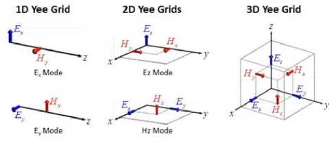
Fig.1. Modality of placing the electric and magnetic field vectors in a 1D, 2D and 3D Yee cell.

Db1 Vj,k =

At   )

V ^ ‘,j,k    1 7

D b2 i,j,k

At

V ^ ‘,j,k   2 7

where A 1 and A 2 represent the two spatial increments that change when calculating the field in a certain point. For example, if only the indices afferent to the axes y and z are changing in the equation, it results that A i = A y and A 2 = A z . For a cubic grid, A x = A y = A z = A and, therefore,   A i = A 2 = A , Cb = Cb2 = Cb and

Db1 = Db2 = Db .

C. Yee's algorithm

The numerical method developed by Yee [9], [13,14], offers the possibility to determine in time and space both the electric field and the magnetic field by solving the two rotor equations. The space in which the field analysis is carried out is divided into cubic cells. As can be seen in

Fig. 1, the E and H components are positioned in the three-dimensional space so that each electric field component is surrounded by four magnetic field components, and each magnetic field component is surrounded by four electric field components. In the space proposed by Yee (a 3D grid), the continuity of the tangential components of E and H is preserved at the interface of two distinct environments, as long as the interface is parallel to one of the coordinate axes of the grid. Therefore, there is no need to specify the boundary conditions at the interface, but the permittivity and permeability must be specified at each point where the field is calculated. Although the Yee algorithm only uses Maxwell's rotor equations, the delivered solutions satisfy implicitly the other two equations (the relations (3) and (4)) due to the location of the E and H components in the Yee grid and the operations with central differences performed [9], [13,14].

The H components are located at the middle of each side of the cube, and the E components are located at the centre of each face of the cube. The components of the E and H vectors are calculated in time, in the leap-frog manner [9], [13,14], as can be seen in Fig. 2. Thus, the E value at a point in space and at a given moment in time is calculated and stored in the memory using the E value at the same point, but at the previous moment, as well as the H values at the previous moment, in points adjacent to the point of interest. The H value is then calculated based on its value in the same point (but at the previous moment) and the E values (previously calculated) in the adjacent points, and the result is stored in the memory. The cycle continues with the recalculation of the E values for the immediately following moment, based on

—*

——

the E and H values previously determined, until the desired moment of time, and so on.

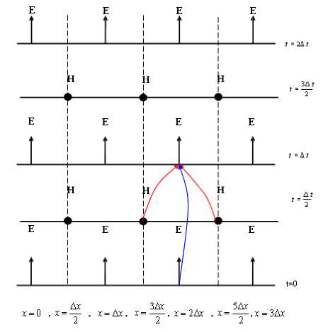
Fig.2. The space-time diagram used to determine E and H in a 1-D space. We see the use of central differences for spatial derivatives and the leap-frog method for temporal derivatives.

D. Electromagnetic field source modelling

In FDTD, we can use as field sources a wide variety of signals [9], [13,14]. The most commonly used are the sinusoidal signal and the Gaussian pulse.

Example of “hard” 1D sinusoidal source:

E(x) = E_o sin ro t

In order to reduce the error, it is used the so-called “soft” sinusoidal source, if the source signal of interest from the source point is added to the previous value of the field.

E(x) = E(x) + E_o sin ro t

The integration step is selected in line with the frequency of the field source.

Example of “hard’ 1D Gaussian pulse:

E(x) = E_o exp

—

c1

)

t I

V   to   J

Example of “soft” 1D Gaussian pulse, if the source signal of interest from the source point is added to the previous value of the field:

E(x) = E(x) + E_o exp

— Ci

( t t )V to J

where we need to model a region that includes an inner field.

In some problems, it is simulated the propagation of the electromagnetic field in open space. In these cases, since our simulation region needs to be limited, we must find a way to “simulate” the open space. These open space limit conditions are called “Radiation boundary conditions” (RBC) [9,10,11,12,13,14,15] or “Absorption boundary conditions” (ABC). The ABCs are necessary to avoid the field reflections on the walls of the integration domain. The most common set of ABC conditions was introduced by J. P. Berenger, named PML (Perfectly Matched Layer) [9,10,11,12,13,14,15]. In case of PML conditions, between the analysed field and the boundary (which remains perfectly conductive) it is inserted an absorbent layer with variable conductivity (the sigma increases linearly – or based on another law – towards the edges of the domain). Thus, if the absorbent layer is sufficiently thick, the waves reaching the end of the domain will be greatly attenuated and the reflections negligible.

Regarding the size of a 3D cell in the Yee FDTD algorithm, it must be small enough to enable obtaining the solution with good accuracy in the case of maximum frequency of interest. The spatial resolution (the distance between 2 successive points) must be selected so that the electromagnetic field does not change significantly from one point to the next one. The spatial resolution or sampling step is a fraction of the minimum wavelength propagating in the grid. To ensure the numerical stability of the algorithm, it is necessary to satisfy a relation [9,10,11,12,13,14,15] between the spatial and temporal increments, A t . In case of constant e and ц , the numerical stability is obtained if:

Example of ‘hard” source 1D modulated Gaussian

pulse:

V m_a/ A ^

E(x) = E_o exp

— Ci

)t j

V   to   J

sin ro t

111 ( H x ) 2 + ( ^ y? f + ( ^ z^ f

Example of “soft” source 1D modulated Gaussian pulse, if the source signal of interest from the source point is added to the previous value of the field:

E(x) = E(x) + E_o exp

—

c1

^

tV to J

sin ro t

E. Boundary conditions, Yee cell size and stability criterion

The boundary conditions refer to what happens to the field component values at the boundaries of the integration domain. The problem does not exist in the limited space, such as a waveguide, a resonator, etc.,

where: v = maximum propagation speed in the grid.

If e and ц are varying, it is more difficult to obtain a stability criterion. The condition (45) imposes restrictions on the temporal increment for the spatial increments.

Once the spatial increments have been set, the temporal increment is selected so as to ensure the numerical stability.

If the propagation occurs only in the x-axis direction,

C A At we denote with A =--- what we will hereinafter call the

Ax stability factor (also called Courant number) [2,3]. The stability factors for the other directions are similarly defined. In general,

_  vx At  vy At  v At

S = x + —  + z

A x    A y    A z

It is demonstrated that if 0 < S < 1, the wave propagating in the grid is not attenuated over time (when the propagation environment has no losses), and if the Courant number becomes greater than one, the amplitude of the wave increases exponentially with each temporal increment [9,10,11,12,13,14,15].

There are some extreme cases:

n + 1        n               n + 1/2       n + 1/2

H y | i = H y | i + D b | i ⋅ (E z | i + 1/2 - E z | i - 1/2 )

The one-dimensional simulation algorithm in case of propagation in the x-axis direction involves the following steps [2,3]:

• a.    If the spatial and temporal sampling is very fine, the numerical solution becomes more and more accurate, but the computation volume and time increase considerably. It can be shown that either the phase speed or the group speed is equal to c (the light speed in vacuum), regardless of frequency (non-dispersive propagation); therefore, the numerical algorithm is non-dispersive [9,10,11,12,13,14,15].

• b.    Magic time-step sampling: c Δ t = Δ x . In this case, the solution obtained is accurate, regardless of the sampling step in time and space.

• c.    Dispersive propagation. This is the most common situation, and occurs if S <1 and Δ x is comparable to λ . It has been noted that the “numerical” wave propagates in the grid with a lower speed than the equivalent “analogue” wave. As     becomes much smaller than      , the

min , numerical dispersion becomes lower and lower.

• 1.    Establishing the dimension of the spatial integration domain.

• 2.    Defining the spatial integration step Δ x .

• 3.    Defining the temporal integration step Δ x in accordance with the signal resolution and excitation. Currently, _{Δ t =} ^{Δ x} , where c is the c

• 4.  Setting  the maximum number of temporal

• 5.  Setting the type, position and, eventually, the

• 6.    Setting the boundary conditions.

• 7.    Initialisation with field update constants, in accordance with the environmental properties.

• 8.    Implementing the field components update cycles.

propagation speed in vacuum or air.

integration steps.

frequency of the source.

III. Fdtd – One-Dimensional Case Study

We will further analyse the propagation of an electromagnetic field into a one-dimensional space. We assume that there are no variations in the y-axis direction, neither of the field nor of the grid geometry. Therefore, the partial derivatives in respect to y and z are null. In this case, the propagation occurs along the x-axis. We also assume that there are no sources of the field ( J      , J        ). The Maxwell’s equations (the source     m,source equations 1 and 2) become:

IV. Description of Gui Application for OneDimensional Fdtd

The GUI application for one-dimensional FDTD is programmed in Matlab [16,17,18,19,20,21] and contains 19 files. For launching in execution, the path to the application folder is set from the Command Window, and then the startup file name is typed. The application's welcome screen is shown in Fig. 3.

∂E  ∂Hy

ε ^z =

∂t ∂x

- σEz µ

∂ H y

∂ E_z

∂t

∂x

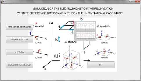
Fig.3. Main interface of the application

∂H  ∂Ey  ∂H

µ z =    - z - σE∂t ∂x    ∂x

,

∂ E y ∂ t

The equations (47) and (48) are rewritten as follows, using finite differences:

n + 1/ 2                    n - 1/ 2

E z | i - 1/2 = C a | i - 1/2 ⋅ E z | i - 1/2 +

+ C b | i - 1/2 ⋅ (H y | iⁿ - H y | iⁿ - 1 )/ Δ x

When pressing the first 3 buttons - Fig. 3, we open word files with information about the FDTD method, Maxwell's equations, and algorithm of the method. When pressing the button “ONE-DIMENSIONAL STUDY CASE”, we open the interface that exemplifies the electromagnetic wave propagation through various environments in “one-dimensional” case – Fig. 4.

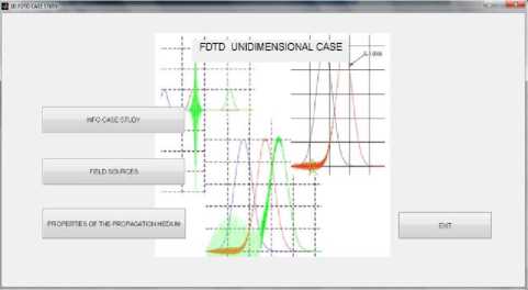
Fig.4. Interface for one-dimensional case study

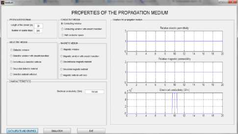
Fig.6. Conducting window

The first 2 buttons open word files with explanations on the case study description and field sources, the third button opens the interface where the type of propagation environment can be selected, and the fourth button closes this interface and opens the start interface. The button “PROPAGATION ENVIRONMENT PROPERTIES” leads us to the interface that enables the setting of some propagation environment properties – Fig. 5.

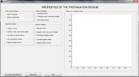
Fig.5. Interface for propagation environment properties

Thus, in the editing fields of the first panel, the length of the propagation domain and the number of spatial steps required for the modelling of the propagation domain and numerical integration are entered. Then, a radio button group is used to select the environment type (conducting, dielectric or magnetic), with variants of environmental models. When selecting a model, a panel with editing fields at the bottom appears to be active, enabling the user to enter the properties of the model in question – Fig. 6. By pressing the button “DATA AND GRAPHIC UPDATES”, we can verify the data integrity, and the charts of relative electrical permittivity, relative magnetic permeability and electrical conductivity versus distance are shown on the right side – Fig. 6.

In the case of the dielectric environment, the following models have been designed [10]: dielectric window, dielectric window with smooth transition, dielectric discontinuity, sinusoidal dielectric, and dielectric with losses. For a conducting environment, the following models have been designed: conducting window, conducting window with smooth transition, half conducting space.

We exemplify the implementation for the conducting environment models – Figs. 6 - 8:

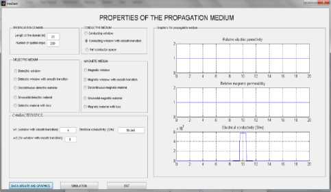
Fig.7. Conducting window with smooth transition

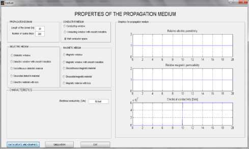
Fig.8. Half space conductor

We can exit from the interface of the one-dimensional model, and by pressing the button “SIMULATION” we reach the interface for the interactive presentation of electromagnetic wave propagation through the environment in question. It is shown the interface for simulating the one-dimensional FDTD – Fig. 9, for the “conducting window” environment model. As you can see, the parameters for spatial integration are transmitted from the environment interface. The spatial step, temporal step and Courant number will be calculated and displayed (that’s why at initialisation they appear as blocked fields). The required values are entered into the editing fields and, by pressing the “SIMULATION” button, we can verify the integrity of data, and the Yee's algorithm is running. The results are presented graphically, in an interactive way – Fig. 9, 10, 11, 12.

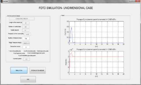
Fig.9. Propagation of electromagnetic field at the moment 3.1667⋅10-9 s

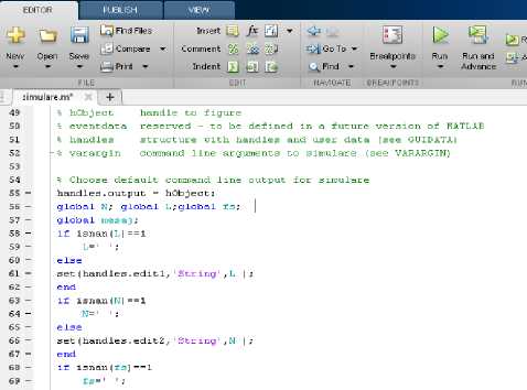
Fig.13. Source code

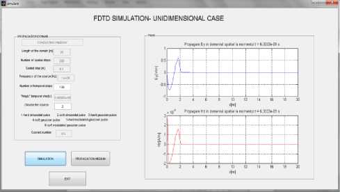
Fig.10. Propagation of electromagnetic field at the moment

6.3333⋅10-9 s

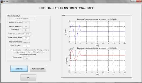
Fig.11. Propagation of electromagnetic field at the moment

1.2167⋅10-8 s

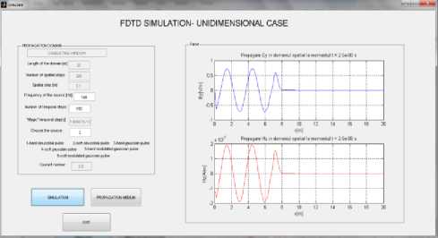
Fig.12. Propagation of electromagnetic field at the moment 2.5⋅10-8 s

Note that (Fig. 13) the student can access the code behind the interface at any time by opening the file in the “Open in GUIDE” design mode with the “Editor” option.

• V. Conclusions

The paper presents a didactic application with graphical interface programmed in Matlab for numerical modelling of the interaction between the electromagnetic field and the matter using the finite-difference timedomain method (FDTD), the one-dimensional case. The method is based on solving the Maxwell's equations in differential form. Basically, the method consists of replacing the differential equations with finite difference equations. The implementation of the FDTD method is based on the Yee algorithm. The application can be used as educational software for the disciplines focused on the numerical methods used to determine the electromagnetic field. It is expected the application to be extended by treating the bi-directional and three-dimensional electromagnetic field propagation cases. Analogically, such teaching interfaces can be made for any course subject to which they fit.

The advantages of using a teaching application with graphical user interface focused on a course subject consist of: active analogical reasoning based on the interactivity of actions, establishing the particular-general and concrete-abstract relationship, facilitating the understanding of the algorithm through interactive viewing of its implementation, real-time visualization of the result of implementation - propagation of the electromagnetic field through the environment in question.

The use of modern teaching methods increases the motivation of students and attractiveness of the courses. The role of the teacher in teaching - learning - evaluation remains still remarkable, and the limits of computer-assisted training can be compensated by alternating the methods and including compensatory methods in the same course.

The proposed method is used by a university year at the Hunedoara Faculty of Engineering and presents a didactic success based on attractiveness, ease of use and understanding.