О спектральной норме прореженных прямоугольных случайных матриц

Introduction and the main result

Let m = m(n), m ^ n. Consider independent zero mean random variables Xj_k, 1 ^ J ^ n, 1 <  к ^ m with ^X²_k = 1 and independent of that

Bernoulli random variables ^7,4 1 + 3 + n, 1 + к + m with E^ = p^. In addition suppose that np_n -4 00 as n -4 00. Then we putp = p_n. Consider the sequence of random matrices

ОН THE SPECTRAL ИПНМ HF SPARSE RECTAHGULAR RAHRHM MATRICES

Institute of Physics and Mathematics, Federal Research Centre Komi Science Centre, Ural Branch, RAS, Syktyvkar Higher School of Economics,

National Research University, Moscow

X - (CjfcXj_k)l^j^_n3^_k^_m. (1)

We denote the non-zero singular values of the matrix X by si > ■ ■ ■ > s„ and define the sample covariance matrix W = XX*.

Let у = y(n) = ^. We are interesed in estimating the maximal singular value si (or spectral norm) of matrix X. The problem of estimating the norm of a random matrix arises in many applications. This topic has been studied by many authors. The case of Wigner matrices or sample covariance matrices has been sufficiently studied. See, for example, the work of Rudelson and Vershynin [1] and the literature to it. Sparse matrices with p_w -4 0 when n -4 00 take a special place. Our motivation for studing the largest singular value of a sparse random matrix is related to the proof of local laws for sparse covariance matrices with "heavy tailed” entries.

The main result of our paper is the following Theorem 1. Let EX,/. = 0 and E|Xy/. |² = 1. Let’s assume that

E|Xyfc|4+6 < Co < 00, for any j, к ^ 1 and for some 6 > 0. Suppose that there exists a positive constant B, such that npn ^ В log” n, where x = э/д5^)- Additionally assume that

\X_jk\ < C^np^-X         (2)

Then for every Q > 1 there exists a constant C = G(Q, d, C_o, Ci), such that

Pr{ si >  C,/np\/logn} Cn ,      (3)

The estimations of the largest singular value for s parse covariance matrices like (3) but without factor ■/logn, with stricter restrictions of moments, is possible to find in [2].

Some applications and proof of the main result

To estimate the spectral norm of the matrix X, we introduce the matrix V

О X X* О ’

where О denotes a matrix of the corresponding dimension with zero entries. Note that

XX* О О x*x and

TrWs = 27W2s.

Let’s consider the estimates of the high order moments of the matrix V. First we note that for g = 2r + 1

ETrV9 = 0.

We investigate q = 2r. Let «2k = ^TrV^2k.

Theorem 2. The following inequality holds for r ^ С(прУ,

Ea_2r<  пр У^ Ea_2sa2r-2_S-2+ s=0

-\-Cnp- —г—E   «2г + GE a<2_T.

(rip)*

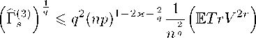
Corollary 1. Under conditions of Theorem 2, for r ^ Co^np^ there exist the constant Ci > 0 depending on C_o such that the following inequality holds

Ea_2r<  СуХпрУ

Proof of Corollary 1 . Let yT = (rip) 2E2ra2r-

Using Young inequality, we can rewrite the result of Theorem 2 as follows уУ ^ _ 4r(l + -——) + r          (rip)*

^уУ + ^су^Уу.

Here from we get the required.

□

Corollary 2. There exists an absolute constant C, s.t. for every t> C,

Pr{si ^ lyTTp y\og n \ ^ exp{—clogtlogn}.

Proof of Corollary 2. Note that (np)* > Glogn. We put r = c log n. It is easy to see that si < пттау.

Applying Chebyshev’s inequality, we get

____ Es2r

Pr{si > nEo2r (ripYXognJ'

Using Theorem 2, we get г                      1    "(‘r

Pr{si > tTnpVlogn} <    <

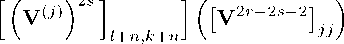
Lemma 1.

ETW2r = ^ (As + Bs) + Zr s=0

where n mm

A.=E=[EEXjkCjkXji^ji X j = l    k=l 1=1

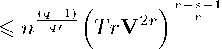
X ((VA)2«1       1 FV2r-2S-21  ,

L              J к-\-тг,1-\-тг J L                Ajj n m

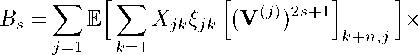
] k-Vn,j

y=i k=\

Proof of Lemma 1. We have the following equality n m

KT-rV» = 2££e.yx>a- [v^2r-‘]_t+„_J y=l k=l

Let’s denote the jth column of the matrix V for j = 1,... , n by Vj. Let

^j = Xge^ + eyVj - ^__XyyeyeJ and vA=V-A,-.         (5)

Using these notations, we obtain

ETrV2r = Ci + C2, where n m

C,i = ££EX,^,fc[vAv2’'-2 j = i k=Y n m j=i k=l

It is straightforward to see that

^-EE^Mdv2-2],.^^.

y=l k=Y

We continue with Gi. Using representation (5), we get

where

= ^^^Хэ^эк [(V^V²^³]

к-\-п,з

G12 = ^^EX^fc y = l fe=l

v^AyV2r"3

-                   J k-Vn,j

Next, it is easy to check that

c_n =            [v«]    [v»-]_u = в,.

3=Yk=Y                   ’

Note that

Gi₂ = 0.

We continue with Gn. Applying again representation

(5), we get

Gn — Gin + Gn2,

where

Cui

-EE ^X₃^₃k [(У^Зу²^⁴]

3 = 3 k=Y

k+n,j

Cyyi

-EE 3k^k [(V^))²A,V^2r"⁴] j=Y k=Y

k+n,j

Using the definition of Ay, we get

where 72772

=^^x^ke3kWv^^^ x j = Yk=Y x \XMs"^33, 72          772772

^s=^2e[^2 ^2 ^jk^jkXji^jiX j = l    k= 1 Z = 1 ,l^k

X Г(У^)2/|       1 rv2r-2s-21

L           J /c+72,Z+72 J LJ

Further, we continue with As as follows я^я^+я^, where 72772

T1’=pEe[E[(v°’)2‘]

j=Y k=Y x fv2"-28-2! , J 33

72          772

A^ =^^Х^зк^ 3 = 3   k=Y

X ^(V^)2S1       1 rv2r-2s-21

L              J к-\-тг,к-\-тг J L                J 33

Using Vkk ^ 0 and V_kk ^ 0 for к = 1,..., n + m and interplacing theorem, we get

A^ < pETrV^2sTrV^2r-^2s-².

We can rewrite it as

-Я^¹) < npEa_2sa_2r__2s_₂. n

Applying Holder inequality, we get 72                772

|Я(²)| <  ^^^(x^e₃k-Ex^e₃k)x j=Y      k=Y

n m m

ся = £££ех,Л^ [(vM)2L 3=1k=\ Z=1

x[V2-yjJ = A2.

x (V^)^2s

Repeating with Gm, we get

72    772

Gm = Bi + ^^EXy^ [(V^)4V2r"5

Continuing this procedure, we get the required. □

Proof of Theorem 2. We start with the estimation of A_s, for s = 1,..., k= . We represent

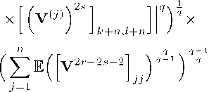
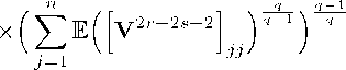
Note that for s = 0,..., [G^] we have q = ^^ > 2. Taking the conditional expectation with respect to V^) and applying Rosenthal’s inequality, we get the inequality

72                    772                                                      q

L                J k-Vn,k-Vn / / j=Y         k=Y

+g9p(np)9-29;J<_2

\ L               J k-Vn_sk-Vn / /

As = As + AS1

This implies that

I^Kr^ + if), where

Note that

< qpy^yTTV'11'

Г^ = C 2npg 52 E i (

— 1 r 2n

2(r—1)

Further,

< ETW2^"1).

Г^²) = q(ripl^V-‘^2,<-A^^4,n^-'5 x

n        m              2(r—1)

x52E" (52 ([(vM) 4

y=l fe=l

x

J кртг^кртг/ /

xE*?|[v^A]J-.

Applying Holder’s inequality and interlacing theorem, we get rW <27^(ETr(V)2(r-1^ <

^^/npqn^ (ETrV2’’) r ,(6)

Г^2) ^Gg^p)1-2^-^^ (ETr^)2^-1)) <

^Сд^р)1"2^-^^ (ETrV2r) " .(7)

Further, we consider A_s. Applying twice Holder’s inequality, we get

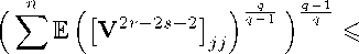
n

^v(52E|[52 52 хзк<зкХр<рх j = l    k=ll = l^l^k

Applying inequality for quadratic forms (see [3]), we get

A_s< nl (fW + f(²⁾ GT®)" x

where fW =qV^V У Gv22 ) V, \ 7-^      \ L J к-\-пД-\-п/ /

Z=1

1У =qXp% (^ар^-ч^-^рх mm        Q q x eV (V Пу22 У2, k=l 1=1 m m ty =y («р^-^-у у y e| У2 I L J /c+n,Z+n k=l1=1

This implies that

УУ q^p^ (np)^~^~^ — (ЕТгУ²’’) ^r . (10)

Finally,

Moreover,

j=i

Combining the estimates (8)—(10), we get

A_s ^ Cnp(^ + S₂ + S₃) (ETr(V)^2r) ~ where

Ei =qn^-2 + r₎

E₂ =q2 ^_Тгр^^-2^-^-^><+д)_тг^-2+г^^-Т=1)

Summing by s = 1,..., [G^], we get

[V]                 1            a 2

As < Cnpn^ —^+t—.i   _ + t—x s=0           V Vn (np)2+^^7

x(ETrV2r) r .

Now we estimate B_s. First we note that B_o = 0.

We can assume that s > 1. We represent B_s in the form n m

^s = 52®[52 52 XjiXjk$_iji£_ijkx y=l    k=\l = \,l^j

The estimation of B_s is similar to the estimation of A_s. We get

IV1               / ,             3

„     1 / r log r r 2

|B_S| <  Спрп'- —+ -— i +

In conclusion, we estimate Z_T. Without loss of generality, we can assume that т is even. First we write

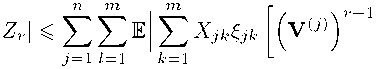
Applying Cauchy inequality, we obtain

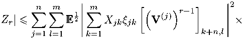
xE^y^,/

Taking the conditional expectation and applying Cauchy inequality again, we get

ЧЕЕ1^ьГ)

Z=1

From here it follows that

П / г i2r—2 \ -

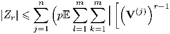
\Z_r\ <  CVp^2 (^ЕГг V^м 7=1

Taking into account interlacing theorem and applying Cauchy inequality, we get cv»^ Тт-м2-2 (e ^ £ | [v^z,/)1 < 4 7 = 1 Z=1

Combining inequalities (6), (7), (11), and estimates of corresponding sums, we get the required.           □

Proof of Theorem 1 . The proof of Theorem 1 follows now from Corollary 2 by choosing t sufficiently large. □