О возможностях и проблемах наблюдений магнитных полей солнца для прогноза космической погоды

One of the most common shared interests of the overwhelming majority of people worldwide is the weather. Knowing what the weather will be like today is sometimes not enough, we often want to know what the weather will be like tomorrow and on subsequent days. The weather forecast has become a vital necessity. For needs of most of the world's population it suffices to know about the state of the surface atmospheric layers (troposphere and stratosphere); however, in recent decades there have appeared areas of human activity in which the term “weather” is used in a much broader sense.

Many global (and often local) processes depend on the state of our star, the Sun, in particular on the number of sunspots. Recognition of the obvious fact stimulated systematic observations of solar activity and attempts to predict it. As early as the middle of the XIX century during studies of spottedness, by analogy with traditional terms of meteorology, terms “solar weather” and “solar meteorology” coined. Over the past half century, intense human activity in space, especially in near-Earth space, at great heights in the atmosphere, and in the subpolar regions, where manifestations of solar-terrestrial relationships are most evident due to peculiarities of Earth’s magnetic field configuration, has raised the question of studying and forecasting conditions in the Sun–Earth system as a whole. This area of scientific and practical activities is now commonly referred to as “space weather” and even “space weather and space climate”. More specifically, the term “space weather” is understood as time-dependent conditions on the Sun, in the interplanetary medium (solar wind), Earth’s magnetosphere, ionosphere, and thermosphere, which affect space-based and ground-based technological systems and can pose hazard to human life and health. According to problems being addressed, space weather research is divided into three types: 1) synoptic solar observations, 2) solar activity forecast, and 3) prediction of interplanetary medium parameters.

It is worthwhile to briefly highlight the history of the origin of the modern term “space weather”. To be fair, it should be noted that this term was first introduced by Alexander Leonidovich Chizhevsky, the famous Russian and Soviet scientist (1897–1964) who is justly recognized as one of the founders of heliobiology – the science that studies the influence of solar activity on terrestrial organisms. Moreover, he put forward an assumption (shared by no means all) that solar activity variations are correlated with historical events – wars, revolutions, natural disasters, etc. Viorel Mihaylovich Lomov [2013] in his book on p. 243 states that for the first time A. Chizhevsky commented on the concept “space weather” in 1915 in his report “Impact of Perturbations in the Solar Electric Mode on Biological Phenomena”. Recognition of scientific contributions of our compatriot is the fact that in 2013 at the 10th European Space Weather Week, the International Alexander Chizhevsky Medal was established. It is awarded to young scientists for space weather and space climate studies.

Unfortunately, A.L. Chizhevsky’s works are ignored in the historical analysis [Cade, Chan-Park, 2015], where it is noted that the term “space weather” was first introduced in the late 1950s and has become commonly used since 1990s, i.e. it is a very young concept, as is the field of science it refers to. Nevertheless, it is a rapidly developing field of science. Results of space weather studies are published not only in traditional astronomical and geophysical journals, but also in specialized publications such as Space Weather (AGU Publication), Journal of Space Weather and Space Climate. International conferences are held regularly, the nearest, the IAU Symposium 335 “Space Weather of the Heliosphere. Processes and Forecasts”, takes place in England on July 17–21, 2017.

The existence of space weather problems allows us to classify solar scientists, heliophysicists, as a special group of astronomers. Without this aspect, they would simply explore an ordinary dwarf star of spectral class G2, a huge number of which exist in our galaxy. It is in the context of solar-terrestrial relations where solar physics occupies a priority position among other research areas of astrophysics and space physics.

As for solar sources (solar drivers) of interplanetary and terrestrial disturbances that are relevant in the context of space weather problems there are several of them, and specific contribution of each of them varies depending on the solar cycle phase and phenomenon under study. The following basic solar drivers are usually distinguished: coronal mass ejections, solar flares, solar wind, solar ultraviolet radiation, energetic particles, and solar radio emission. The most effective in exciting disturbances are certainly coronal mass ejections (CME), solar flares, and energetic particle fluxes accompanying both the phenomena. Also of particular relevance is the information about radio emission and luminosity (specifically in the shortwave spectral range, variations in which may be as high as 10 % depending on solar activity versus 0.1% variations in total and visible radiation).

The solar magnetic origin of most space “troublemakers” on Earth was proved as far back as the middle of the XIX century when a correlation was revealed of the intensity and number of geomagnetic storms with the number of sunspots. The giant geomagnetic storm of 1859 is well known. It produced intense aurora and caused malfunction of telegraph. Richard Carrington attributed this storm (though with great caution, saying «One swallow does not make a summer»!) to the strong white-light solar flare that occurred in the vicinity of a large active region on September 1, 1859 [Carrington, 1859]. A classic example of the close solar-terrestrial relation is the March 13–14, 1989 geomagnetic storm (comparable in strength to the Carrington event), which was preceded by a powerful CME on March 9. During this storm, contact with many satellites was lost, and an electrical blackout occurred in Quebec, Canada, which cost $100 million. Noteworthy among relatively recent catastrophic events is the October 29, 2003 magnetic storm, which caused malfunction in electrical networks in South Africa and Sweden [Cid et al., 2014].

Ground-based and space-based systems for monitoring solar processes have been created and actively developed in civilized countries. In Europe, there is the Space Situational Awareness Program (SSA) of the European Space Agency []; in the USA, the U.S. National Space Weather Strategy and National Space Weather Action Plan (. To be fair, it should be noted that the first steps in establishing “solar patrol” in the context of space weather effects (on ionospheric disturbances and, consequently, on radio wave propagation) were made by Germany as far back as 1940s during the Second World War. In particular, in the interests of the German Air Force in the Alps, a network of three solar observatories was built up in Germany and one observatory in Austria.

Important and in some cases principal source of all these drivers is a magnetic field. Ultimately, it is the energy stored in the magnetic field along with dynamic phenomena in the convection zone and outer atmospheric layers that is realized in solar processes. Observations of solar magnetic fields are urgent and absolutely necessary to solve most problems of space weather forecast. Data on such fields are used both directly, for example for calculating parameters of the solar corona and interplanetary medium, and indirectly, for example to search for their relation (proxy) with luminosity variations. The purpose of this review is to analyze the current state of solar magnetic field observations. Applicability will be explored (not fully, of course) of various series of solar magnetic field observations (individual magnetograms and synoptic maps) for predicting solar wind parameters and geomagnetic activity indices.

By no means all of numerous solar observatories in the world, even those with large telescopes designed primarily to study fine structures, are capable of conducting full disk monitoring of magnetic fields; whereas this is a necessary condition for the use of magnetograms in space weather problems. The following table gives basic information about solar observatories equipped with full-disk magnetographs. The new-generation telescope STOP [Peshcherov et al., 2013] is installed in the Mountain Astronomical Station of the Central Astronomical Observatory of RAS (MAS CAO) near Kislovodsk because this observatory makes most regular observations; some results of these observations are reported in this review. In actual fact, ISTP SB RAS on commission from the Fedorov Institute of Applied Geophysics (IAG) has made three identical instruments to create a network of three observatories, which, along with Kislovodsk, includes Ussuriysk and Baikal Astrophysical observatories.

The table shows that the instruments differ both in the method for separating spectral lines of interest in a spectrum (spectral selector may be a spectrograph, birefringent filter (BF) or interferometer) and in spectral lines in use. Moreover, spectrograph-based instruments scan disk (by meander if a photomultiplier or a CCD linear detector is used as a photodetector, or by one-dimensional displacement of a solar image across the entrance slit along one of the spatial coordinates α, δ in case of a CCD matrix), while filter — and interferometer-based instruments have to scan a spectral line profile or measure in selected parts of the profile when observing the full disk. Each of these methods has merits and demerits. Another important difference between magnetographs is spatial resolution that varies from several tens of pixels per disk along one of the coordinates to a few thousands.

Especially noteworthy is the zero-level control in observing magnetic fields at different telescopes [Demidov, 1996]. The most obvious would seem to be the method using a nonmagnetic line (WSO, FeI 512.4 nm line). However, the adjustment of the spectrograph to another wavelength necessary for this method poses particular problems (and it is absolutely inaccessible for filter magnetographs). In general, the identity between values of zero shifts in working and nonmagnetic lines is valid only at a certain accuracy level. In many respects, a more reliable method using a phase half-wave plate (STOP) eliminates most instrumental problems, but its disadvantage is that in high spatial resolution observations, insertion of a large-size polymer film causes degradation of image quality and increases scattered light. The third method of zero level control (SOLIS) is indirect, unlike the aforementioned first two, and involves a special, additional processing of data within various assumptions such that when averaged over long time intervals, signals from vast areas of the solar disk with weak magnetic fields should be zero.

Basic information on instruments whose magnetic field observations are used for space weather forecast

Instrument	Location	Wavelength selector	Working spectral line in use, nm	Angular resolution (arc sec)	Dimension of full-disk magnetogram X×Y pixels
WSO (Wilcox Solar Observatory)	Stanford, USA (λ = 122° W, φ = 37.4° N)	Littrow spectrograph	FeI 525.02	90×180	21×11
SOLIS	Tucson, USA (λ=111° W, φ = 32.2° N)	Littrow spectrograph	FeI 630.15 FeI 630.25 CaII 854.2	1×1	2K×2K
GONG	Global network of 6 stations	Michelson interferometer	NiI 676.8	8×8	256×256
SOHO/MDI	Lagrange point L1	Michelson interferometer	NiI 676.8	2×2	1024×1024
SDO/HMI	Geosynchronous orbit, 36 thousand km, λ = 122° W, 28° inclination	BF Lyot filter + Michelson interferometer	FeI 617.3	0.5×0.5	4K×4K
SMAT HSOS	Beijing, Huairou, China (λ =116°, φ = 40.3° N)	Tunable BF Lyot filter	FeI 532.4	2×2	992×1004
STOP MAS CAO	Kislovodsk, Russia (Λ=42.6°, φ=43.7° N)	Littrow spectrograph	FeI 630.15 FeI 630.25	33×6	59×294
STOP SSO	Sayan, Mondy Russia (λ=101°, φ=51.6° N)	Littrow spectrograph	FeI 525.02 and others	91×91	21×21

The table provides information about ground-based and space-based instruments. Advantages and disadvantages of observations of each type are discussed, for instance, in [Balasubramaniam, Pevtsov, 2011; Pevtsov, 2016]. Clearly, ground-based and space-based observations complement each other, and ground-based data are not, under any circumstances, to be written off. Unlike space-based data, ground-based data are longterm (this is essential for synoptic programs) and relatively cheap. Moreover, ground-based instruments can be upgraded at any time with the advent of new technologies. The obvious disadvantages – the distorting effect of Earth's atmosphere and time dependence (observations are not made at night) – can be compensated by using adaptive optics and by setting up a network of similar telescopes. Finally, these ground-based observations are essential for calibrating and testing space-based instruments.

SOME INFORMATION ON METHODS AND MODELS FOR CALCULATING SOLARWIND PARAMETERS AND GEOMAGNETIC ACTIVITY INDICES INFERRED FROMSOLAR MAGNETIC FIELD OBSERVATIONS

The Sun affects Earth both directly, via electromagnetic and corpuscular emission, and indirectly, via various processes in the interplanetary space. Sources and characteristics of the solar wind (SW), which is a connecting link between the Sun and Earth, have been extensively studied, in particular by Russian scientists. Kovalenko presents a very comprehensive review on publications as well as his own important results in his monograph [Kovalenko, 1983], which has not lost its relevance today. Under stationary conditions, the quiet solar wind flows out of subequatorial regions of the solar corona at a velocity of about 400 km/s with a frozen-in magnetic field, forming a quasi-stationary structure whose main element is heliospheric current sheet (HCS) – the boundary between polarities of the interplanetary magnetic field (IMF). The solar wind velocity from polar coronal holes is much higher and reaches 800 km/s. The quiet solar wind is modified by processes that occur in active regions and coronal holes, thus leading to deformation of HCS, CME, and complex dynamic interactions between various fluxes in the interplanetary medium. Geomagnetic activity depends on Earth’s position relative to HCS (that is, in general, substantially distorted with respect to the solar equatorial plane) since this determines whether the geomagnetic field orientation coincides with the IMF B z component or is opposite to it. In the latter case, we deal with reconnection processes and more active changes in the magnetosphere. The change in orientation of the geomagnetic field with respect to IMF leads to semiannual geomagnetic activity variations, known as the Russell–McPherron effect [Russell, McPherron, 1973]. Specific conditions of the IMF–magnetosphere coupling, which modify the Russell–McPherron effect, occur during spring and autumn equinoxes [Cliver et al., 2000], causing a combined “equinox effect”.

Attempts have been repeatedly made [Pudovkin et al., 1977; Ponyavin, Pudovkin, 1988; Obridko et al., 1996; etc.], which are currently of only historical interest, to find empirical relations of the observable magnetic field parameters, derived from full-disk magnetograms, with solar wind (orientation and magnitude of IMF components, velocity, density, time of propagation to Earth’s orbit) and geomagnetic activity indices.

Later on, more complex and sophisticated forecasting methods were worked out, including complex threedimensional magneto-hydrodynamic (3D MHD) models. In problems of predicting SW parameters near Earth at a distance of 1 A.U. from the Sun, two approaches are distinguished: the first involves computing background, quiet SW and corona; the second, calculating dynamic phenomena such as CME. Initial conditions for complex models of the second approach are simplified models devised for the first approach. The first approach most commonly relies on the Potential Field Source Surface (PFSS) model [Schatten et al., 1969; Altschuller, Newkirk, 1969 Levine et al., 1977; Hoeksema, 1984; Rudenko, 2001]. This model assumes that the coronal magnetic field is potential (this forced simplification means that photospheric and chromospheric currents, which, of course, exist in reality, as well as forces associated with gas pressure are ignored) and becomes completely radial at a certain level above the photosphere. This level is called the source surface. Its height is a free parameter; it is usually taken to be 2–2.5 radius from the Sun’s center. The polarity structure at this level is set fixed and is carried out by the solar wind radially to the outer heliospheric regions. The raw observational material for the calculations are synoptic maps of the radial field derived from daily magnetograms, in which the field is recorded along the line of sight (longitudinal field), by recalculating in the approximation of predominantly vertical direction of the magnetic field in the photosphere (see discussion of this issue in the recently published paper by Leka et al [2017).

Note that along with PFSS there are other models that are partially or completely free from PFSS’s shortcomings. A detailed discussion is beyond the scope of this paper, and therefore I restrict myself only to listing some of them. This, in particular, the CSSS model (Current Sheet Source Surface) [Zhao, Hoeksema, 1995], Adaptive Mesh Refinement Solar InterPlanetary space-time Conservation Element and Solution Element Magnetohydrodynamic model (AMR SIP–CESE MHD model) [Feng et al., 2012a, b], and global model of the solar corona MAS (Magnetohydro-dynamics Around a Sphere) [Mokic et al., 1999; Riley et al., 2003].

To compute solar wind parameters from the PFSS calculations of the solar corona, Wang and Sheeley [1992] and Arge and Pizzo [2000] worked out an empirical model, called WSA model, which is widely adopted for space weather prediction. This model is employed as a first approximation and boundary conditions in modern threedimensional MHD models [Hayashi et al., 2015].

The most “advanced”, state-of-the art predictive code for calculating solar wind parameters, which is used in the real-time mode in the Space Weather Prediction Center (SWPC) of the National Oceanic and Atmospheric Administration (NOAA) in Boulder, is Enlil, named after the supreme Sumerian deity, the god of wind. Enlil was devised by Dusan Odstrcil (University of Colorado, Boulder) in collaboration with other researchers [Odstrcil, Pizzo, 1999a, b; Odstrcil et al., 2002, 2003, 2004]. It relies on the three-dimensional MHD model of the heliosphere, which describes the solar wind plasma motion and the time variation of the solar wind magnetic field. The inner boundary of the model is at 20–30 radii from the Sun, and its parameters are usually determined by WSA calculations. The outer boundary can reach 10 a. u. and more, but for practical purposes, calculations for Earth’s orbit are of major importance. The model operates in a range of ± 60° in heliolatitude. The latest modification of WSA-Enlil, when the review was being written, was WSA-Enlil+Cone [Mays et al., 2015]. It is capable of predicting conditions of the interaction between Earth and CME observed by coronagraphs (including STEREO) at distances up to 20 solar radii, the geometry of CME propagation in interplanetary space approximated by a cone. An example of operation of WSA-Enlil+Cone is given in Figure 1, which represents a screenshot made when downloading a site.

However, it should be noted that no matter how complex and versatile methods and models for predicting space weather parameters would be, they cannot ensure 100% accuracy [Mays et al., 2015]. One reason for this situation lies in the reliability of raw data themselves.

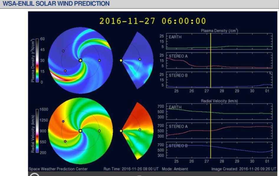
Figure 1. Screenshot of the display on a computer screen when downloading results of prediction of plasma density (top panel) and radial velocity (lower panel) of the solar wind by the WSA-Enlil+Cone model from the NOAA/SWPC website []. Results of calculations for Earth (some sectors to the right), as well as for two STEREO satellites

PROBLEM OF UNCERTAINTY IN OBSERVING SOLAR MAGNETIC FIELDS:FULL-DISK MAGNETOGRAMS AND SYNOPTIC MAPS

Magnetograms from different observatories may differ quite significantly. This is demonstrated by the example of the analysis of full-disk magnetograms in [Demidov et al., 2008], where there is also a fairly detailed bibliographical review of the problem of comparing solar magnetic field observations in different observatories and spectral lines. An extensive analysis of synoptic maps from data obtained at seven observatories has been carried out in [Riley et al., 2013]. The conclusion of that work is very unfavorable – data from different observatories can differ very considerably, from 4–5 up to 20 times (see upper right panel in Figure 9 in [Riley et al., 2013]). Moreover, these ratios vary with time and with position on the solar disk (depending on heliolatitude). The last fact is particularly important for space weather problems since magnetic fields in the polar regions have a strong effect on calculation results. Groundbased (mainly from SOLIS as well as from the Mount Wilson Observatory’s magnetograph) and space-based observations of solar magnetic fields were compared, in particular, in [Pietarila et al., 2013].

Wang, Sheeley [1995] have laid the foundation for a discussion of the possible influence of problems in solar magnetic field measurements on space weather problems, specifically on calculations of the structure of the solar corona and solar wind parameters. The authors proposed using the correction factor found by Ulrich [1992] to correct magnetograms from the Wilcox Solar Observatory (WSO).

K=4.5–2.5sin2ρ, where ρ is the heliocentric angle. Later [Ulrich et al., 2009], this formula was modified:

K=4.15–2.82sin2ρ, and in this form it was used for one of the recalibrations of SOHO/MDI magnetograms. However, the authors of [Svalgaard et al., 1978; Svalgaard, 2006; Demidov, Balthasar, 2009, 2012] spoke out against such correction of observations in the FeI 5250 Å line (in this very line, WSO makes measurements). The conclusion drawn in [Svalgaard et al., 1978; Svalgaard, 2006] about the need to correct WSO data by a constant (in time and disk) factor of 1.85 because of saturation of the magnetograph signal was confirmed in [Riley et al., 2013].

Let us discuss in more detail the results of [Hayashi et al., 2016], which analyzes differences in calculations (performed in the potential approximation, i.e. by the PFSS model) of the heliosphere structure and solar wind parameters in Earth’s orbit, using synoptic maps from four observatories: WSO, GONG, SDO/HMI, and Huairou Solar Observation Station (HSOS). The analysis used the Carrington rotation 2144 (from November 21 to December 19, 2013) during maximum solar activity. One reason for choosing this Carrington rotation is Earth’s heliolatitude close to zero. This allows us to eliminate differences between magnetic field effects in subpolar regions, coronal holes in which, as is well known, affect calculations of the heliosphere.

The question about magnetic field observations in polar regions of the Sun, which have a significant effect on the configuration of the solar corona and interplanetary magnetic field, is really crucial. The interpretation of magnetic field observations at large distances from the solar disk center is a scientific challenge (see, e.g., [Solanki et al., 1998; Demidov et al., 2015]). Observations of polar regions are also complicated by the fact that they periodically (every six months) are outside the field of view (Earth’s heliolatitude effect). Therefore, the absence of data for the Sun’s polar regions should be compensated somehow, for example by extrapolating low-latitude fields [Petrie, 2015]. In some cases (the ADAPT model – Air Force Data Assimilative Photospheric Flux Transport [Arge et al., 2010]), polar magnetic fields are restored through calculations by flux transport models.

The spatial resolution of synoptic maps from the four observatories being greatly different, all data were reduced to the resolution of WSO maps, i.e. the number of points on a synoptic map was 72 (longitude) and 30 (sine latitude). The authors of [Hayashi et al., 2016] applied an important procedure – respective average (over the entire map) values of Δ B were subtracted from all synoptic maps to correct the unbalanced magnetic flux. This procedure for correcting zero-level shift had practically no effect on WSO and HMI data (Δ B =–0.08 and –0.11 G respectively), but markedly affected HSOS data (Δ B =–1.13 G) and GONG (Δ B =–1.21 G). This very fact may explain the rather inaccurate forecasts made with WSA-Enlil+Cone, where basically GONG data are used.

The use of this procedure for zero-level shift correction led to a situation that results of calculations of coronal holes in regions with magnetic field lines open to the interplanetary space proved to be very different (and in the case of GONG and HSOS, they were totally different). This is clearly seen from Figure 2 borrowed from [Hayashi et al., 2016] (Figure 4 in the original source). In this figure, dark color indicates regions with coronal holes. The upper panel shows calculations without correction of synoptic maps, and the bottom panel, those with zero-level shift correction. It can be seen that panels for HMI and WSO differ slightly, and panels for GONG and HSOS have little in common.

Also illustrative in [Hayashi et al., 2016] is Figure 10, which demonstrates the comparison between real observations and results of calculations of the radial magnetic field component near Earth’s orbit for different data series with and without zero-level shift correction. It is easy to see that without correction (the validity of which, as done in [Hayashi et al., 2016], in my opinion, is far from obvious), the calculation results for GONG and HSOS differ considerably from experimental data.

The existence of significant problems with the zero-level control at SMAT/HSOS (Solar Magnetism and Activity Telescope) has been discovered with direct involvement of the author. Several experiments using a halfwave phase plate (in much the same way as it has been done for many years [Demidov et al., 2002] at STOP of the Sayan Solar Observatory) revealed [Demidov et al., 2016] significant zero-level shifts in SMAT magnetograms, being different for different positions on the solar disk. Figure 3 illustrates the comparison between HSOS and SDO/HMI data without (left panel) and with (right panel) zero-level control. Apparently, after zero-level shift correction, HSOS data agree much better with SDO/HMI data.

Thus, we can conclude that proper consideration of numerous instrumental effects, which can distort real observational data, especially consideration of zero-level position, is necessary. Therefore, observations at the instruments, where such a procedure receives appropriate attention (at WSO the zero level is controlled using measurements in the nonmagnetic line FeI 5124 Å, at STOP/SSO, using a half-wave plate), should be regarded as more reliable. This is also confirmed by Figure 4 that presents the results of comparison between calculated and actually observed values of the solar wind velocity in Earth’s orbit, which were taken from [Tlatov et al., 2016]. These observational data were acquired at STOP in Kislovodsk.

It is particularly important to know the solar wind velocity in Earth’s orbit as it is proved (see, e.g., [Newell et al., 2007, 2016] and references therein) that this parameter correlates well with geomagnetic activity indices. The comparison between observed solar wind velocity values calculated in different models (in particular, [Owens et al., 2008; McGregor et al., 2011]) revealed great differences. This initiated recalibration of the model calculations.

Recently, in the discussion about the influence of raw observations on calculation results in the context of space weather problems, in addition to comparison of different data sets, a new aspect has arose which is related to peculiarities of construction of synoptic maps (observations made on different days are used to build one map).

The effect of such uncertainties is demonstrated to be significant [Bertello et al., 2014; Pevtsov et al., 2015]. In the end, the idea was discussed [Weinzierl et al., 2016; Pevtsov et al., 2016] of launching a spacecraft with a full-disk magnetograph to Earth’s orbit at the Lagrangian point L5 to assess reliability of space weather forecasts and increase their lead time. There is no doubt that if this project (which is, of course, very difficult because the L5 point is at a distance 10 times farther than L1 from Earth, which imposes limitations on the useful load mass and telemetry) is implemented, the space weather program will rise to a fundamentally new level. Scientific instruments for space vehicles at the L1 and L5 points, including full-vector magnetographs with sufficiently high spatial (angular) resolution, are thoroughly discussed in [Kraft et al., 2016]. The angular distance of 60° between the line from the center of the Sun to the point L5 and the Sun–Earth line would provide 67 % coverage of the entire solar surface, and, compared to 3–4 days when observed only from Earth and from L1, would ensure a greater, up to 6–7 days, lead time of observations of active regions and hazardous processes.

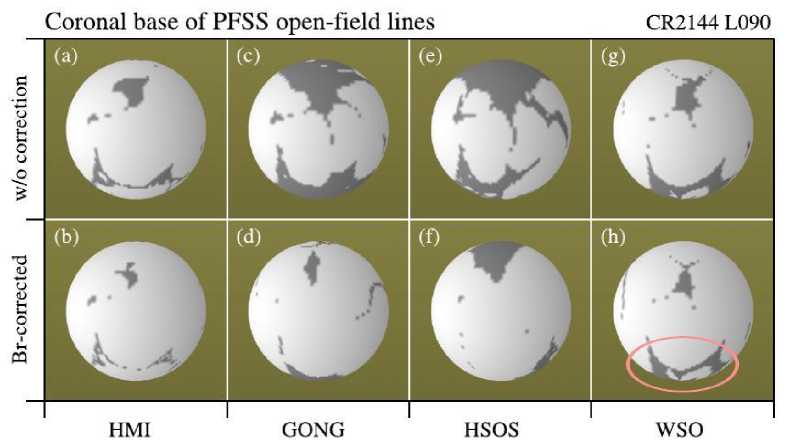
Figure 2. Regions of coronal holes on the solar surface (calculated in the PFSS approximation), from which open magnetic field lines emanate. Results of calculations made with synoptic maps from the four observatories without (top panel) and with (bottom panel) zero-level shift correction. Especially noticeable are substantial changes caused by correction of GONG and HSOS data. The figure is from [Hayashi et al., 2016]

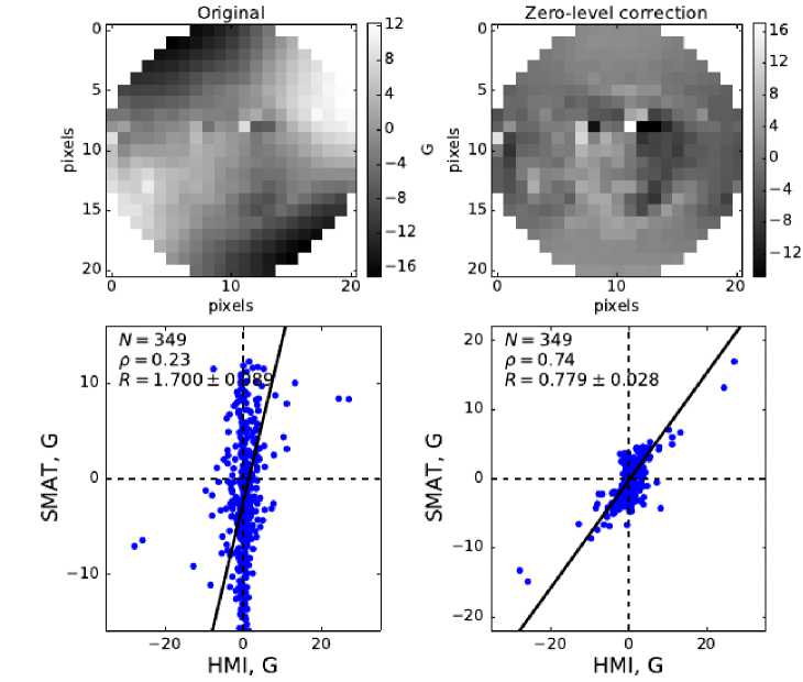
Figure 3. Efficiency in consideration of the zero-level shift effect on SMAT/HSOS observations. At the top to the left is the original magnetogram, and to the right is that corrected for zero-level shift. At the bottom is the comparison between the SMAT–SDO/HMI magnetograms (scatter plots): to the left is the initial SMAT magnetogram, to the right is that after zero-level shift correction

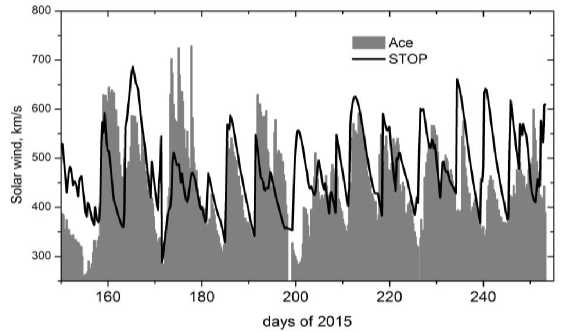
Figure 4. Comparison between measurements of the solar wind velocity at ACE (Advanced Composition Explorer) at the point L1 and values computed from observations made at STOP in Kislovodsk. The figure is from [Tlatov et al., 2016]

DISCUSSION AND CONCLUSION

Unfortunately, in Russia space weather research has almost no its own experimental and observational basis and necessary funding. Numerous discussions and projects have remained just talks or decisions only on paper and as yet have no practical implementation. It is especially sad because there was time (1960–70s) when in this respect, as in many others, Russian science was world-first and enjoyed a certain prestige. However, something is still being done despite the current crisis, and this is encouraging.

In terms of the subject matter of this review – the use of solar magnetic field observations for space weather problems – it is pleasant to note that in addition to the long-standing and best performing Solar Telescope for Operational Predictions (STOP) of the Sayan Solar Observatory, a network of similar new-generation telescopes with much higher spatial resolution and shorter time of recording of full-disk magnetograms has recently been established. Such instruments are installed in Ussuriysk, Irkutsk, and Kislovodsk.

The analysis carried out (by no means complete, of course) suggests that full-disk magnetic field observations are essential and very effective in solving space weather problems. More research is needed to find the most reliable data. A new line of research seems promising – the use of not only longitudinal magnetograms and synoptic maps of radial field, but also full-vector magnetograms and respective synoptic maps for space weather forecasting [Liu et al., 2017]. There is no doubt that new and interesting results will soon be obtained in this direction.

I would like to thank reviewers for positive reviews and valuable comments and advice, which, I hope, allowed me to greatly improve the article.

The work was done partially under the Fundamental Research Program No. 7 of the RAS Presidium “Experimental and theoretical studies of objects in the solar system and planetary systems of stars. Transitional and explosive processes in astrophysics” and the Fundamental Research Program of RAS SB II.16.1 “Fundamental problems of space weather processes, including processes on the Sun, in the interplanetary space, Earth’s magnetosphere and atmosphere” (Project II.16.3.3 “Astrophysical instrumentation and methods”).