On a Class of Dual Risk Model with Dependence based on the FGM Copula

Author: Hua Dong, Zaiming Liu
Journal: International Journal of Information Engineering and Electronic Business(IJIEEB) @ijieeb
Article in issue: 2 vol.2, 2010.
Free access
In this paper, we consider an extension to a dual model under a barrier strategy, in which the innovation sizes depend on the innovation time via the FGM copula. We first derive a renewal equation for the expected total discounted dividends until ruin. Some differential equations and closed-form expressions are given for exponential innovation sizes. Then the optimal dividend barrier and the Laplace transform of the time to ruin are considered. Finally, a numerical example is given.
Dividends, dependence, barrier strategies
Short address: https://sciup.org/15013056
IDR: 15013056
Text of the scientific article On a Class of Dual Risk Model with Dependence based on the FGM Copula
Published Online December 2010 in MECS
It is well known that the classical risk process has been studied profoundly, e.g. Asmussen[1], Gerber and Shiu [2, 3], Dufresne and Gerber [4]. For the classical risk model, it is assumed that the inter-claim times between two successive claims and the claim amounts are independent. Such an assumption may be inappropriate in real world. To avoid the restriction, some risk models with dependence structure between inter-claim times and claim sizes are proposed. Among them, Albrecher and Boxma[5] have proposed an extension to the classical compound Poisson risk model in which the distribution of the time between two successive claims depends on the the previous claim size. Albrecher and Teugels [6] considered an risk model with arbitrary dependence structure between the inter-claim times and the subsequent claim size through a copula. In Boudreault et al.[7], they assumed that the claim size depend on the inter-claim times.
The barrier strategy was first studied in De Finetti [8]. Barrier strategies for the compound Poisson process risk model have been studied in detail by numerous authors, e.g. Dickson and Waters[9], Landriault[10], Lin et al.[11]and Lin and Pavlova[12].
Recently, there has been growing interest in a model which is dual to the classical risk model. See Asmussen [1], Albrecher et al. [13], Avanzi et al. [14], Avanzi and Gerber [15], Ng [16], Song et al. [17] and references therein. Avanzi et al. [14] considered the expected total discounted dividends until ruin for the dual model under the barrier strategy by means of integro-differential equation.
Avanzi and Gerber [15] extended some results of Avanzi et al. [14] to a dual model perturbed by diffusion. Ng [16] generalized the study of Avanzi et al. [14] to a dual model with dividend threshold strategy. Here, we aim at extending some results of Avanzi et al. [14] to a dual risk model with dependence structure which is based on the Farlie-Gumbel-Morgenstern (FGM)(see Nelsen [18]) copula.
Consider the dual model
N(t)
U^t) — и — ct + У^ X; — и — ct + S(t), t > 0, where u > 0 is the initial surplus, c > 0 is the constant rate of expenses and S(t) represents the aggregate gains up to time t. The innovation number process №>o}is a renewal process with inter-innovation times Wl^i, where Wl^i is a sequence of strictly positive and independent random variables (r.v.) with probability density function (p.d.f.) Jw and distribution function (d.f.) F\ у. Throughout this paper, it is assumed that И has an exponential distribution with mean 1 /A. The innovation size (gains) r.v.’s №Ъ>1 , where Xj corresponds to the amount of the j th innovation, are assumed to be a sequence of strictly positive and independent r.v.’s with a common p.d.f. fx , d.f. Fx , mean Mx and Laplace transform fx . We assume that {(ВД forms a sequence of i.i.d. random vectors with joint p.d.f. fx.w^x,^ for t > 0 and z > 0 . It is clear that the increments {Х,-сИА,7 = 1.2,...} of the surplus process are still independent. To ensure that ruin will not occur almost surely, we assume that д = XE(X{ - clV;) = Xpx - c > 0, г = 1,2, • • • . (1) Furthermore, we assume that the joint distribution of (X, W) is defined with the FGM copula (see Nelsen [18]), which is defined by
C(u, v) = UV + 611(1 — u)v(l — v), —1 < 6 < 1. (2)
Given (2), the joint distribution function of Fx.w^i () is defined by
= FxkxWwW
Thus, the joint p.d.f. is given by fx,w(x,D = c(Fx(x^Fw^fxWJwW
= fxWwm (1 + 0(1 - 2Fx(x))(l - 2FtH0)) -
In this paper, we assume that the dividends are paid according to a barrier strategy, say with the parameter b > 0. Whenever the surplus exceeds the barrier b, the excess is paid out immediately as a dividend. Let Fj,(f) be the modified surplus process with initial surplus IW = U under the above barrier strategy b .
Let V(w,b) = E[J^ e~5tdD(t)] denote the expectation of the discounted dividends until ruin with the boundary condition V(O:b) = 0 , where T = inf{< > 0 : UbW = 0}(T = oo if ruin does not occur) is the time of ruin and 6 > 0 is the force of interest to discount the dividends.
Noticing that
V (u; b) = и — b + V(b; b), u > b, (5) we will mainly discuss the model for 0 < u < b.
The paper is organized as follows. In Section 2, we start by deriving an integro ‐ differential equation satisfied by V(u;b) . Then the integro ‐ differential equation leads to some differential equations and closed form expressions for exponential gains. In Section 3, we discuss how we can use the method of Laplace transforms to obtain the expected total discounted dividends. A renewal equation is also given. In section 4, the optimal dividend barrier is considered. The Laplace transform of differential equation leads to some differential equations and closed form expressions for exponential gains. In Section 3, we discuss how we can use the method of Laplace transforms to obtain the expected total discounted dividends. A renewal equation is also given. In section 4, the optimal dividend barrier is considered. The Laplace transform of the time to ruin is studied in Section 5 for exponential gains. Finally, a numerical illustration is given in Section 6
II Expressions for V(u;b)
Theorem 2.1 For 0 < u < b, V(u;b) satisfies the following integro ‐ differential equation
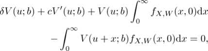
where
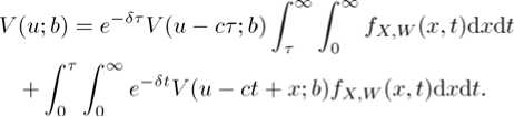
Proof. Choosing a time т small enough such that u — ст > 0, one obtains
Differentiating the above equation with respect to T and then letting т — 0 yield (4).
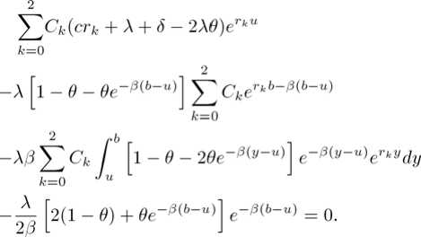
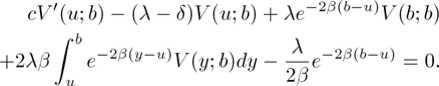
Corollary 2.1 For 0 < u < b, if the gains are exponentially distributed with mean 1/^9 , then V(u;b) satisfies the following integro-differential equation cV\u; b) + (A + <5 - 2A0) V(u; b)
-A(l - 0 - 0e-3(6-u))e"w-u)V(b;b)
-X3 / (1 - 0 - 20e-/3^-u))e-^(y-“) V(y; b^dy
-^(2(1 - 0) + 9e-^b-u^e-^b-^ = 0. (7)
Corollary 2.2 If the profits are exponentially distributed with p.d.f. fx^ = 0e 91, x>0 and e e [-1.0) и (0.1), then V(u; b) satisfies differential equation cV"\u; b) + (A + 6 - 3c/3)K"(u; b) + 2532V^u; b)
-9(2A + 3d' - 2c3 - X6W4u; 6) = 0, (8)
for 0 < u < b.
Proof. Applying the operator ^,-т^-ад to (7), then we obtain (8).
From (8) and the boundary condition У\0;Ь^ = О, we have
V(u;b) = Y^CkeTkU1 k—^
^ [-1,0) и (o.i), (9)
where rk(k = 1.2,3)are the solutions of the equation _ A/3(l - 0) 2X93 e equation cs + A + 6 - 9_s + 5^^- (10)
To determine Ck = Ск^ , we insert (9) into (7) and obtain
By matching the coefficients in (11) one obtains
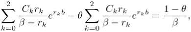
which is the coefficient of де-0(Ь-и) , and
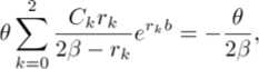
which is the coefficient of Ле-29(Ь-и) . Combining with the boundary conditionV(O;b) = О, we have fc=O
cV"(u; b) + (A + 6 - 23c)V'(u; b) - 236V(u; b) = 0, for 0 < и < b.
Proof. Setting 9= 1 in (10), we have
Define мas the coefficient matrix of the system (12) ‐ (14) and the column vector п= (/3, -1/2/3,О)т. Let Mi be the matrix obtained from п.М by replacing its г th column by 77 for i=l,2,3. Denote the determinant of a matrix by det(-) . Then, we have Ci = (det(M))~* det(M,+i), i = 0.1,2, provided that det(M) / 0. Some careful calculations give
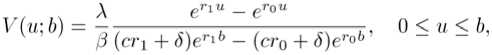
By applying the operator(^-2/3)to this equation, we obtain (15). From the boundary condition V(O;b) = 0 and (15), it follows that
Д er\u _ erou
23 (cti + <5)ег'ь - (сто + 6)er°b' 0 < и < b, (16)
where r0 < 0 < n are solutions of equation ex2 + (A 4- 6 — 23c)x - 236 = 0. (17)
e( } [(/3-n)(2/3-r2) (/3-r2)(2/3-r,)]
хпг2е(г1+г2)6
+l(/3-r2)(2/3-r0) (/3 - r0)(2/3 - r2)
хгог2е^го+г2^ь
+l(/3-r0)(2^-n) (/3 — Г1)(2/3 — r0)
хг1Г0е(г1+го)6
det(M1) = <№^+да
"(^^) + г/з^-го)^06’
^ = 3(^ + 20^
_(^(2/3-n) + 23(9 - ’ det(M3) = ^+9^ г^Г1еПб
/3(2/3-ri) 2/3(/3 -n)
-----------+-----------)r2er2b.
1<3(2/3-r2) + 23(3- Г2У 2
Corollary 2.4 If the profits are exponentially distributed with p.d.f. fxW = ^e 91, x > 0, and 0 = 0, then for 0 < и < b
cV'4m b) 4- (A + 5 - 3c)v'(u; b) - 36V (u; b) = 0, which is (3.2) in Avanzi et al. [14]. Thus
where ro < 0 < n are solutions of equation ex2 4- (A 4- 6 - 3c)x — 36 = 0. (18)
Let
Tu,b
= inf{f > 0,
U(t) >b.O
V(u;b) = ^[е-^'ЧГ^б), which means that
5[e-$T„.i.] = V(U;b)V(b;b)-x.
Remark 2.1 When 9 € (0.1), one can show that
A 4- A , д ,
--< tq < 0 < ri < 3 < r2< 23;
c
When 9 6 [-1.0), one can show that
A + 6
--< To < 0 < ri < 3 < 2/3 < r2. c
In a word, (10) has one negative root and two positive roots.
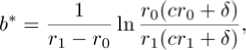
Corollary 2.5 If the profits are exponentially distributed with p.d.f. fx^x) = 3e 91, x > 0, then for 9= I
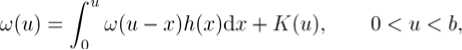
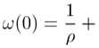
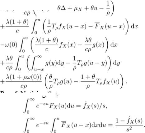
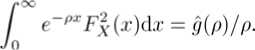
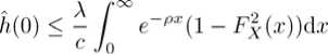
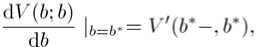
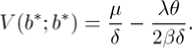
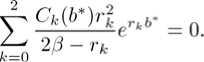
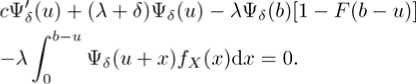
£?[e- erlU _ erou prYb _ pTOb ’ where ГО, Г1 are solutions of character equation (17); for 0 = 0, the expression for E[e- equation (18). For9 6 (0,1)U[-1,O), ^[е-^ил У,к=оскег,-Ь Corollary 2.3 If the profits are exponentially distributed with p.d.f. fx(.x) = 3e 91, x > 0, and 6= 1, then V(u; b) satisfies differential equation III Renewal equation For notational convenience, we denote the Laplace transform of a function. £ by Ф) = Г е ex^(®)da: for Re(.s) > О, and Fx^ = 1 - Fx^. In order to get the Laplace transform of V (u; b) , we replace the random variable и by z — b — и as in Avanzi et al. [14]. Denote W(z;b) = V(b — z;b), for 0 < z < b. (19) Then it follows from (7) that cW\z-,b) + XW^O;b)Fx(zXl - 9FX^ +A Г W(x;bKl + 9 - 20Fx(z - x^Jx^ - x)dx (l-0Fx(x))Fx(x)dx = O, with boundary condition W^F) = V(b;b), (20) W(b;ty = 0. (21) We extend the definition of w(~; 0) by (20) to z > 0 and denote the resulting function by ШМ. Then сш'^ - (A + 8)*) + Aw(0)Fx(2)(1 - 0Fx(z)) +A [ w(x)(l - 9 + 20FxU - x^jx +xj (1 - 0Fx(x))Fx(x))dx = 0. with w(0) = V(6; 0) and w(b) = 0. Taking Laplace transform on both sizes of (22) and rearranging it, one obtains (0) mw^hh^ _ AH( ) Ш S = --—-------2--=------—, cs - (A + 6) + A( 1 + 9Hx (s) - XOg(s) where ZX= Fx(x)(l-Fx(x))d.r, ./o g(x) = 2Fx(x)/x(x), Л _ /x(s) - 1 + sgx - 6(1 - sw(0))(g(s) - /x(s)) ~ S s2 Let = XJ~ e—Xx2/x(x)dx ° A /o°° e"sxx2(g(z) - /x(x))dx Д(8) = cs - (A + 6) + A(1 + 9Hx^ - Xeg(s'), where -4(s) is the denominator in (23). It is obvious .4(0) < 0, .4(oc) = linis-юо .4(s) = oo. When 0e l-1.0o), the second derivative of -4(s) is positive, otherwise the second derivative of -4(s) is negative. Under any circumstance, -4(s) has a unique positive zero, which is defined as P- P must be the zero of the numerator of (23). Some careful calculations lead to 1 // - А0Д w 0 - - + -- P d Remark 3.1 When the gains are exponentially distributed with mean 1//3 , we have Л5) = 3+^»9(s) = ^; - 2ТЙ. Replacing s with — s in Д(б), we know that Д(б) is the negative root of the expression on the left‐hand side of (10). In this case, P = -ro. Remark 3.2 When 0 = 0 , (23) and (24) can be simplified to (7.3) and (7.8) in Avzani et al. [14], respectively. For any integral real function ( , denote Tr<(x) = J” e-r<»-^<(g)dg, r € C. (see Dickson and Hipp [19]). Inverting the Laplace transform in (23) lead to the following Theorem: Theorem 3.1 w(n^ satisfies the following renewal equation with boundary condition w(b) = 0, (26) p - X6^ where h(u) = A(1 + e^Tpjx^Jc - XOTpg^/c, Proof. Noticing that Inverting (23) leads to the renewal (25). Since p is the zero of Л(8) = 0 , it must also be the zero of the numerator in (23). Substituting p into the numerator of (23, noticing А(^ = О and some careful calculation lead to (27). (26) is obvious since (21). Remark 3.3 For (25) to be a defective renewal equation, it remains to show that к(О) < 1. By the property of operator тг, we have ^-^-T0TpJxW - ^-Т0Трд^ Х(1 + О)р, - , .. Хбр, .. с- (1 - /х(рУ) - -^(1 - д^ х А(1 + 0) - хе ---тр) + —дкР) ср ср ср - + — Г e-^FxWxWx ср с Jo с Jo where we have used For — 1 < 0 < О, it follows from (28) that А А Г™ /i(O) <--- e-pxFxMdx ср с Jo Fx(x)dx< 1. The last equality is due to the positive security condition (1). For О < 0< 1, we have When /о°° е"^! - F^^dx < рх , (25) is also a defective renewal equation. at for each u. Thus 9V(u;b) _ |б=ь- -°, and hence that IV The optimal dividend barrier In this section, we adopt a similar approach to those used in Avanzi et al.[5] and Avanzi et al.[6] to consider the problem of the determination of the optimal barrier. Let Ь* be the optimal value of b, then УМ is maximal where у'(ь-,ь) denotes the left derivative ofV(u;b) at и = b. Using (3), we can get У'(Ь*—;Ь*) = 1 = У'(ЬЧ;Ь*). (31) This phenomenon is the high contact condition in finance literature and the smooth pasting condition in literature on optional stopping problem. Setting u = b = b* in (4) and using (30), we obtain According to Avanzi and Gerber[6], we can set ш(°) = л ~ ^ and obtain the function W(2) by ' ' О ZpO ' ' ^ inversion of its Laplace transform. Then b* is the zero of ш(~), and VM*) = w(b* - u), 0 < u < bV Remark 4.1 When the gains distribution is exponential distribution with mean 1/0 and 9 € [-1.0) П (0.1), we can easily get the optimal dividend barrier b* as Avanzi and Gerber[6] did. It follows from (30) and (9) that С'к(Ь*) = О, к = 0,1,2. (33) Now differentiating (12) and (13) with respect to b, settingb^b*and applying (33), we get y> Ck(,b*y^еГкЬ. = 0 (34) Then solving the linear system forCo^VCi^VC^ composed by (14), (34) and (35), we can get the b* which satisfies v(6’) = 0. Remark 4.2 When the gains distribution is exponential distribution with mean 1/^3 and9= 1, there is a closed form expressions for b*. From (16) we obtain where Го and Г1 are the solutions of (17) with Го < 0 < П . V Laplace transform of the time to ruin In this section, we consider the Laplace transform of the time of ruin T for the surplus process /7j,(f) under the barrier strategy. Let Ф,(ы) = ^[е-6т|Г6(0) = u], u > О, be the expected present value 1 due at the time of ruin. As a function of d , it is the Laplace transform of T . As a function of и, it is easy to see that Фй(и) = 1 for и< О. Noting that Фд-(и) = Ф5(Ь)(и > Ь) , we only discuss Фб(и) for О < и < Ь. Theorem 5.1. Suppose that the profits are exponentially distributed with p.d.f. /x(®) = 0е-9\ х > О , then фд(м) satisfies the following integro‐differential equation c^uj + (А + 8^М - А(1 + 0)ФЙ(6)7(6 - и) +А0Фй(и)(1- Г2(6-и)) -А(1 + 0) ^$(u + x)J^dx Jo +А0 I Ф5(и + x'lg^dx = О, Jo for 0 < и < 6. (36) Proof. The proof is similar to theorem 2.1. Corollary 5.1 When the gains distribution is exponential distribution with mean 1//3 and 9 6 [-1,0) П (0.1), ФДи) satisfies the following differential equation сФ^и) + (А + <5 - Зс^)Ф^(и) + 2/32<$Ф5(и) -3(2А + 3<$ - 2сЗ - А0)Ф^(и) = 0. (37) proof. Applying the operator(Д-Д^-гДto (36), we obtain (37). Then from (37) and the boundary condition Фй(0) = 1, we have ФбМ-^Окв1^ 0 У ег,Ь = 0(39) £ = °-(40) Гк -2/3 From the boundary condition ф5(0) = 1, we have 2 £^ = ь(41) к=О Then solving the linear system composed by (39), (40) and (41), we can get Do. DbD2. Corollary 5.2 When the gains distribution is exponential distribution with mean 1//3 and 9 = 0. Фд(и) satisfies the following differential equation сФ"(и) + (А + 6 - сЗ)Фд(и) - /ЗАФ^н) = 0. (4.1) Proof. Setting 9 = 0 in (36), we have By applying the operator (м ЭД to this equation and after some careful calculation, we obtain (42). It follows from the boundary condition Фй(О) = 1 and equation (42) that (3 - тоухег‘ь+г»и -(3- Г1)гоег°ь+г1" 5 U (3- ro)rier*b - (3 - г1)гоег°ь ’ О < и < Ь, where Го and Г1 are the solutions (18.) Corollary 5.3 When the gains distribution is exponential distribution with mean 1/3 and 9 = 1, ФДи) satisfies the following differential equation сФд(и) + (А + 5 - 2с/3)Ф^(и) - 2^Ф<(и) = 0. (43) Proof. Similar to Corollary 2.3. From the boundary condition Фл(О) = 1 and equation (43), we have Ф»(и) = Г1(2/3- г0)еГ16+г»и г 1(2,3 - г0)еГ1Ь г0^3 - rYKob+rxU го^З ~ гх')егоь О < и < Ь. where Го and Г1 are the solutions (17) VI Numerical illustration In this section, we illustrate the effect of dependence. Let $х^ = е-, then the covariance between X and И7 is given by Cov(X,I¥) = fS2(2,l) , where В(х,у) = J01^-1(l-<)y-1df . This implies that (X, W) is positive correlation when е > о, otherwise the verse. SetА = 2, с= 1.1, 6 = 0.1.By comparing table I–V, we find that V(,b; b) is a increase function about ь; when ь is a determine constant V^u;^ is a increase function about и. The optimal dividend barrier ь* decrease as 0 increase. Table VI‐IX shows the probabilities thatU (f) reaches ь from и (и < Ь) without ruin occurring. When b — и is a determinant constant, the probabilities increase as tz increase. When и and b are constants, the first exit probabilities increase as 0 decrease. Table I INFLUENCE OF 6 ON К(и; b), b = 1 Table II INFLUENCE OF^ ON У^Ь') b=2 1u 9=1 9=0.5 9=0 9=‐0.5 0.1 0.0491 0.1270 0.5559 1.3081 0.5 0.2516 0.5708 2.3453 5.2404 0.8 0.4130 0.8466 3.3374 7.2099 1 0.5267 1.0075 3.8768 8.2080 1.2 0.6464 1.1516 4.3393 9.0214 1.5 0.8392 1.3373 4.9198 9.9897 1.8 1.0513 1.4848 5.3970 10.7573 2 1.2054 1.5588 5.6719 11.2052 u 9=1 9=0.5 9=0 9=‐0.5 0.1 0.0707 0.0999 0.3554 0.7067 0.5 0.3629 0.4362 1.4993 2.8484 0.8 0.5956 0.6235 2.1336 3.9553 1 0.7595 0.7156 2.4784 4.5489 Table III INFLUENCE OF^ ON V(«; Ь^, b = 3.5 1u 9=1 9=0.5 9=0 9=‐0.5 0.1 0.0257 0.1290 0.6837 1.7196 0.5 0.1318 0.5824 2.8841 6.8866 1 0.2759 1.0393 4.7675 10.7750 1.5 0.4395 1.4103 6.0502 13.0736 2 0.6313 1.7217 6.9750 14.5328 2.5 0.8615 1.9881 7.6897 15.5526 3 1.1426 2.2106 8.28840 16.3462 3.5 1.4902 2.3681 8.8127 17.0272 Table IV INFLUENCE OF о ONV(u;bVb = 4 u 0=1 0=0.5 е=0 в=‐0.5 0.1 0.0204 0.1238 0.6817 1.7255 0.5 0.1049 0.5591 2.8756 6.9102 1 0.2196 0.9983 4.7534 10.8188 1.5 0.3498 1.3564 6.0324 13.1182 2 0.5204 1.6605 6.9545 14.5825 2.5 0.6856 1.9285 7.6670 15.6058 3 0.9094 2.1700 8.2596 16.4020 4 1.5307 2.5574 9.2822 17.7170 Table V INFLUENCE OF^ ON У(»; 6), b = 4.5 1u е=1 е=0.5 е=0 0=‐0.5 0.1 0.0162 0.1172 0.6682 1.7032 0.5 0.0832 0.5926 2.8188 6.8208 1 0.1742 0.9458 4.6595 10.6720 1.5 0.2775 1.2856 5.9131 12.9486 2 0.3987 1.5750 6.8170 14.3939 2.5 0.5440 1.8317 7.5155 15.4040 3 0.7215 2.0672 8.0963 16.1899 4 1.2145 2.4839 9.0987 17.4879 4.5 1.5575 2.6388 9.5734 18.0926 Table VI First passage time 0 = 0 1u b=2 b=3 b=4 b=5 b=6 1 0.6939 0.6113 0.5808 0. 5683 0.5629 2 1 0.8810 0.8370 0.8190 0.8113 3 1 0.9501 0.9296 0.9209 4 1 0.9785 0.9693 Table VII: First passage time е = 1 u b=2 b=3 b=4 b=5 b=6 1 0.3215 0.1374 0.0659 0.0336 0.0178 2 1 0.4275 0.2050 0.1046 0.0554 3 1 0.4796 0.2446 0.1296 4 1 0.5101 0.2703 Table VIII First passage time 0 = 0.5 u b=2 b=3 b=4 b=5 b=6 1 0.6502 0.4850 0.4310 0.4023 0.3861 2 1 0.7967 0.7071 0.6579 0.6331 3 1 0.8844 0.8264 0.7912 4 1 0.9307 0.8924 Table IX First passage time О - -0.5 u b=2 b=3 b=4 b=5 b=6 1 0.7467 0.6935 0.6786 0.6732 0.6715 2 1 0.9222 0.9021 0.8950 0.8926 3 1 0.9757 0.9680 0.9655 4 1 0.9921 0.9575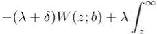

References On a Class of Dual Risk Model with Dependence based on the FGM Copula
- S. Asmussen, Ruin Probabilities, World Scientific,Singapore, 2000.
- H. U. Gerber, E. S. W. Shiu, “The joint distribution of the time of ruin, the surplus immediately before ruin, and the deficit at Ruin”, Insurance: Mathematics and Economics, 1997, 21: 129-137.
- H. U. Gerber, E. S. W. Shiu, “On the time value of Ruin”, North America Actuarial Journal, 1998, 2: 48-78.
- F. Dufresne, H. U. Gerber, “The surplus immediately before and at ruin, and the amount of the claim causing Ruin”, Insurance: mathematics and Economics, 1988, 7: 193-199.
- H. Albrecher, O. J. Boxma, “A ruin model with dependence between claim sizes and intervals”, Insurance: Mathematics and Economics, 2004, 35:245-254.
- H. Albrecher, J. Teugels, “Exponential behavior in the presence of dependence in risk Theory”, Journal of Applied Probability, 2006, 43(1): 257-273.
- M. Boudreault, H. Cossette, D. Landriault, E.Marceau, “On a risk model with dependence between interclaim arrivals and claim sizes”, Scandinavian Actuarial Journal, 2006, 5: 265-285.
- B. DeFinetti, ” Su un'impostazione alternativa della teoria collettiva del rischio”, Transactions of the XV International Congress of Actuaries, 1957, 2: 433-443.
- D. C.M.Dickson, H. R. Waters, “Some optimal dividend Problems”, ASTIN Bulletin, 2004, 34: 49-74.
- D. Landriault, “ Constant dividend barrier in a risk model with interclaim-dependent claim sizes”, Insurance: Mathematics and Economics, 2008, 42: 31-38.
- X. S. Lin, G. E. Willmot, S. Drekic, “The classical risk model with a constant dividend barrier: Analysis of the Gerber-Shiu discounted penalty function”, Insurance: Mathematics and Economics, 2003, 33: 551-566.
- X. S. Lin, K. P. Pavlova, “The compound Poisson risk model with a threshold dividend strategy”, Insurance: mathematics and Economics, 2006, 38: 57-80.
- H. Albrecher, A. L. Badescu, D. Landriault, “On the dual risk model with tax payments”, Insurance: Mathematics and Economics, 2008, 42: 1086-1094.
- B. Avanzi, H. U. Gerber, E. S. W.Shiu, “Optimal dividends in the dual model”, Insurance: Mathematics and Economics,2007, 41: 111-123.
- B. Avanzi, H. U. Gerber, “Optimal dividends in the dual model with diffusion”, ASTIN Bulletin, 2008, 38: 653-667.
- A. C. Y. Ng, “On a dual model with a dividend threshold”, Insurance: Mathematics and Economics, 2009, 44(2): 315-324.
- M. Song, R. Wu, X. Zhang, “Total duration of negative surplus for the dual model”, Applied stochastic model in business and industry 2008 24: 591-600.
- R. B. Nelsen, “An introduction to Copulas”, second edition, Springer-Verlag, New York, 2006.
- D. C. M. Dickson, C. Hipp, “Ruin probabilities for Erlang(2)risk process”, Insurance: Mathematics and Economics, 1998, 22: 251-262.
