On application of weak regeneration in simulation of complex inventory control systems

Inventory control management is very important for every complex manufacturing or logistic distribution enterprise. Efficiency and effectiveness of inventory control management can greatly minimize the financial losses. The objective of controlling and managing the inventories is to determine and maintain the right amount of investment in the inventory and the manufacture.

One can create some safety stocks of inventory for decreasing costs associated with the possible shortage. On the other hand, the supplementary stock increases the holding costs. According to this, the typical problem that usually comes up is precise determination of the optimal volume of the ordered items as well as orders frequency. In this context an inventory order policy can generally be divided into two parts: determining the order quantity, i. e. the amount of inventory that will be purchased or produced with replenishment or determining the reordering point, when the inventory is low but can still meet the customer demands and new supplies arrive just in time before the last item is sold.

When analyzing a stochastic inventory control model [7], [8], [9], the following objective can arise: minimization of average total costs per time unit, and, as a consequence, minimization of waiting times for a demand at every location/echelon.

In this context the authors pick out the following problem: to estimate the average total waiting time for a demand in the system for a regeneration cycle and confidence interval limits for this time. A period between two consecutive regeneration points is taken as a regeneration cycle for the system. At these points a demand passes through the system without any collision with other demands, i. e. the system is idle at such points. However, this requirement is too restrictive. Moreover, efficiency of such type of simulation can be quite low, as a location cannot start to service the next demand while the service of the current demand is not completed. To avoid this, the weak regeneration points for a location/echelon will be considered, i. e. such points that a demand passes through the system without collision at every location/echelon. In other words, a location/echelon can be busy at a previous instant, but will be idle at a current instant when a demand tries to enter this echelon.

To be able to estimate the regeneration points, the inventory control system is analyzed from the viewpoint of a queuing system. The weak regenerative approach is used, which has been investigated for simulation and estimation of steady-state characteristics of queuing networks [1], [5], [6], and an inventory control system [7].

The paper is arranged as follows. The main definitions of regeneration phenomena are stated in the first part. The model of the complex inventory system under consideration is described in the second part. The third part is devoted to the regeneration structure of the given system.

DEFINITIONS OF REGENERATION PHENOMENA

Consider a d -dimensional right-continuous realvalued stochastic process X = {X(t), t ∈ T} , where T = [0, ∞ ) or T = N, with state space {R ^d , B}.

The process X is called weak regenerative with regeneration points β = { β _l}_{l ≥ 1}, if for each l , the postprocess { X ( t ), t ≥ β_l , ( β_l+k – β₁ )_{k ≥ 1}} does not depend on the pre-history { X(t) , t <  β_{l – 1} , β ₁, …, β_l }, l ≥ 2 and its distribution is dependent on l ≥ 1.

The sequence { β _l}_{l ≥ 1} forms the embedded renewal process { α _l = β _l+1– β_l}_{l ≥ 1} of regeneration cycle lengths (we assume a zero-delayed case whe n β ₁ = 0), and l -th regeneration cycle of the process X is defined as

G i = { X ( t ) : P i <  t <  P i _{+ 1}; a = P i _{+ 1} - P i } .

In a weak regeneration case the cycles G_l are identically distributed and dependent in general. In most typical cases dependence in a queuing process may be reduced to one-dependence, in which case { G_l+k }_{k ≥ 2} and { G_{l – k} }_{0≤k≤ l – 1} are indep en dent, but G _l, G _l+1 may be dependent. The process X is classic regenerative if the cycles { G _l} _{l ≥ 1} are independent.

Assume that a w eak limit X _∞ of the basic regenerative process X exists. To estimate stationary characteristics r = Ef ( X _∞ ), we introduce the i. i. d. variables

P l + 1 ^{- 1}

• Y , = 2 f ( X k ) , U = Y - ra , , l > 1. (1) k = в ,

Assuming E ( Y ₁ + α ₁)² < ∞ . It is the weakest condition for confidence estimation based on the regenerative approach to be held, [4]. Then the following well-known ratio r = EY ₁/ Eα ₁ holds.

In a classical regeneration case, the Central Limit Theorem (CLT) gives the following asymptotic (1 – 2γ)% confidence interval for r rN

± Z zY

SNl 1

AT 1/2 --- '

N a « J

where rN = YN/αN, αN, αN and YN are sample means of {α1} and {Yl}respectively, z is selected so that P(N(0,1) ≤ zγ) = 1 – γ, and tγhe sample variance S2 (N)= YN + rNaN - 2rNSN ^ a2with probability 1 as N → ∞, where a2 = E U2 = VarY1 + r 2Vara1 - 2r • cov(Y1, a) (3)

As we have discussed the weak regeneration in a queuing system is usually reduced to the one – dependence, in which case,

E ( U 1 U 2 ) = cov Y - r a 1 , Y 2 - r a ₂ ) = cov ( Y 1 , Y , ) - r cov ( a ₂, Y 1 ) (4)

Thus, the CLT for the one-dependent variables gives us the following (1 – 2 γ )% confidence interval for r

У rN

±

_Zy ^S ² ( N ) + 2 ( t 1 ( N ) - r N t 2 ( N ))

Nn«n

where t ₁( N ), t ₂( N ) are standard estimates of cov ( Y ₁, Y ₂), and cov ( α ₂, Y ₁), respectively, [1], [3]. Also with probability 1 as N → ∞ ,

S ² ( N ) + 2 ( 1 1 ( N ) - r N t 2 ( N )) ^ a ²,       ⁽⁶⁾

where now σ ² = Var U ₁ + 2E( U₁U₂ ) [2].

MODEL DESCRIPTION

We consider the complex inventory control system which has to satisfy a demand for a final product and represents a manufacturing and assembly process for a subassembly. The system contains m echelons, every i-th echelon consists of ni locations (producers), except the first echelon (a retailer), i = 2, .„, m; n 1 = 1, 2”i ni = M. Each location produces only one component. This system is the so called convergent multi-echelon system and is characterized by the property that a location is supplied by one or more previous locations (predecessors), and supplies exactly one location (a successor), as is shown on Figure. Here the first number by every location is the number of an echelon, and the second one is the number of a location within the echelon.

The described system is able to produce K types of production. Each type of production demands a set of components which are produced at corresponding locations. For every type of production the retailer defines the route containing the required components (locations) and the amount of inventory materials supplied for every producer. The retailer immediately forwards a demand to the producers with respect to a given route. In other words, there are K routes in the system.

The order lead time consists of the production times at each location and transshipment times between locations plus possible delays (waiting times and delays of materials supply). The interarrival times of demand orders to retailer are assumed to be independent and identically distributed random variables (i. i. d.). The same we assume for production times at locations, materials supply delays and transshipment times between locations.

^{Echelon m} Echelon m – 1 Echelon 2 Echelon 1

Producers           Sub-                             Sub-                Retailer (Final

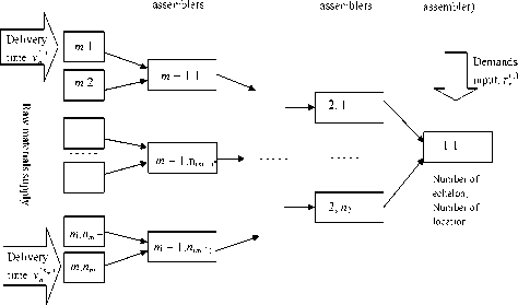
Multi-echelon manufacturing system

To estimate the performance of the given system we assume the following cost factors: cost function C_z ^{( i )} for transshipment from i -th echelon to ( i – 1)-th echelon per time unit, waiting time cost C_w ^{( i , j )} per time unit at location j of echelon i , j = 1, …, n_i , i = 2, …, m and shortage cost C_v ^{( j )} , j = 1, …, n_m . We remark that waiting time cost means cost for delays at locations due to collisions with other demands. Shortage cost is cost for delay of demands at the retailer because of inventory materials deficit.

For steady state expected cost TAC we have now:

m ⁿ i m               ⁿ m

TAC = 22 C W^{l , j )} W + 2 C Z) Z + 2 C

( i , j ) v ^,

i = 1 j = 1

i = 2

j = 1

wher e Z is the average transshipment time per loc a tion, V is the average delay time per location, and W is the average waiting time per location.

REGENERATIVE STRUCTURE

As for estimating the average values used in TAC the weak regeneration approach is applied, let’s describe the regenerative structure of the given inventory control system.

Let tn,1) be the arrival time of n-th demand at echelon i, r(‘) = t(‘) -t(‘), i = 1, .., m, i. i. d. interarrival , n n+1 n ,            , , , times of demands at echelon i with rate λi.

Let Sn^{1 ,} j ) be the production time of n -th demand at location j of echelon i , i = 1, .., m ; j = 1, .., m i , S^¹ the production time of n -th demand at first echelon. We assume that all locations of i -th echelon have identical production time with rate ц = 1/ ES(' ) .

Let zn' ) be the transshipment time of n -th demand between echelon i and echelon ( i -1), i = 2, …, m , and v nj ) be the delay time of n -th demand due to materials delivery to j -th producer, j = 1, …, n_m .

We denote I n = ( 5 _n⁽‘ ),..., 5 n^m ) ) "the route of n -th demand, I_n ∈ I_K , where I_K is a set of routes, 5^ = ( 5 n^ , a , 5^- ) ) , i = 2, ., m , and S^ j = 1 , if j -th location of i -th echelon is part of n -th demand route, and 0 otherwise.

If the known condition

• A.

P - = --------^ 1, - = 1, a ,m,           (7)

max ц j j=la, n- holds and moreover

Pт >5 if max S (j + X v (^{j )} V- j ) + z (° | + S ^ | > 0., (8)

• ^        i = 2 ^ ^j = L a , n          j = 1      J             J J

then a positive recurrent renewal process of classical regeneration points of the system exists, and the system is idle at such instants. However, such points are generally too rare in real inventory systems, and the following weaker assumption

• ⁽¹⁾    ._ С⁽ П                    ^{(1)                        ( m} . j )         ⁽ j ) ^{( m} . j )

P(T1 > S1 )> 0, PT1 > max ((S1   + v 1 5 )> 0, j =, a' nm                                        (9)

P (r , ^(,) >  max ( S , ⁽ j ⁾ 5 „^<' ^j ) ) > 0, i = 2, a , m - 1

seems more suitable. Under assumptions (1), (3) one can construct weak regeneration points so that a demand can cross the system without collisions.

To motivate our interest to _m the weak regeneration approach, we remark that if 5 P - <  1 , then condition (2) holds and classical regeneration may be acceptable for estimation [6]. However, in a complex inventory control syst _m em with a large number of echelons the assumption E ^p - >>1 seems more natural.

An important problem which arises in simulation practice is how to identify efficiently weak regeneration points during simulation. Fortunately, one can indicate a wide class of the renovating events that allow us to do it for a given inventory system.

Consider the process W n = ( W_n ⁽¹⁾, a, W _n ^(m ) )} , W n¹ ) is the current unfinished workload when n -th demand arrives at echelon i , i = 1, …, m , n ≥ 1.

Fix some vector a = ( a ₁, ..., a_m ), a_i > 0, i = 1, …, m (and suppress the dependence on a_i in notations). Define the following events

^ ⁽ a ) = k” >  a 1 ;

S ' ¹* >  a ₂, max ( S n ( i • j ) • S (i • j ) ) > a. i = 3,..., m ;

j =1, a, П, V7

W n1 + S na — 1 < a 1 ;

• ⁽¹⁾    I C⁽¹⁾             ( ^m )                        ( ^m , j )       ( ^m , j )

w „ 1 + S „ 1 + w „ 1 + max S„, • o_     <  a. + a₃ ;

n — 1 n — 1 n — 1                         n — 1 n — 1              12

• j = 1, ^a , n m

Wn°) + Sn—)1 + Wnm + max (S^^) • 5^”;^))+

• j 1, ^a , ⁿ m

^{( m —} 1)                           ^{( m —} 1, j ) ^{( m —} 1, j )

• ⁺ W n — 1 ⁺ max ( S n — 1 • ⁵ n — 1 ) < a 1 ⁺ a 2 ⁺ a m ^;

j = 1, a- ⁿ m — 1

...

W n — + S n — )1 +i5 (W n ^l— ) + max ( S n —- j ) • 5 n —/ ) ) )< i m a , } .

i = 2 ^X              j = 1, a , n,                          ' - = 1

The main idea underlying the events is that on the event Ω _n demands n , n + 1, … cross the inventory system along the given route without collision with demands 1, 2, …, n – 1. The presence of the “barriers” a_i is actually necessary to guarantee one-dependence of the regeneration cycles [1], [5], [6].

Define recursively the points во a) = 0;

p^1-^ = min { ^ : t k. >  p n^a ) , event Q -—, occured } , n > 0.

Then points { p n ^a ) } form a positive recurrent renewal process of weak regeneration points for the current workload process W = {W _n , n ≥ 0}.

Unfinished current workload W(-) at each ech-n elon i can be easily computed through well-known Kiefer-Wolfowitz recursion which for our case has the following form:

W_n + ) = W n^{(- )} + max ( S n^{- , j )} • 5 _n ^{( - , j )} ) — t ( ^{- )} ) + , n >  0. '               j = 1, a-, n- '                         '             l

CONCLUSIONS

In the present paper the authors investigated stochastic processes stipulating behavior of the complex inventory control system. The regenerative structure of the given system was described. The weak regeneration cycle length and 95 % confidence intervals for average waiting times of demands were estimated using the proposed approach. Obtained regeneration points can help a decision-maker in controlling the stochastic process of demand service. One can postpone a demand service starting time until the next regeneration point so that the total waiting time for this demand will be minimal, and average total costs per time unit will tend to minimal as well. It results in a smoother business operation and an optimized utilization of resources and manpower.

* Работа выполнена при поддержке Программы стратегического развития (ПСР) ПетрГУ в рамках реализации комплекса мероприятий по развитию научно-исследовательской деятельности на 2012–2016 гг.