On calculation of moment of resistance in canals of low-rate centrifugal pumps

High-speed low-rate centrifugal pumps with rotor angular pump units of liquid-propellant engines of low traction and velocity ω of up to 10000 rad/s have a wide use in the turbo- aircraft energy installation. They a have wide range of

• *This research is sponsored by state grant MK-1826.2008.8 and state program «Scientific Potential of Higher Institutes of Education Development» № 2.1.2/802.^*

operating conditions e. g. if the rotor angular velocity ® = 3000 : 10000 rad/s, the value V /ю is equal to 1 •Ю" ⁷ m ³ under the Reynolds number Re _m >  10 5 . The feed decrease in such pumps parallel with rotor angular velocity increase leads to V /ю decrease below value V /to = 1 • 10 ⁶ m ³. It is a rating value for closed-type impeller rotary pumps [1]. Therefore high-speed rotary pumps with semi open-type impeller are widely used.

For the low-rate centrifugal pumps (LCP) the moment of resistance in the pump canal is half of the total resistance moment in the LCP case. For this reason the problem for determining the moment of resistance is of great importance.

In this paper we speak about the pump canal. The flow in the canal is divided by a convention of the core and the boundary layer; the liquid movement in the core is axisymmetrical: flow streamlines are closed annular lines. When the liquid passes between two coaxial cylinders [2] the circumferential velocity U is distributed according to UR – constant. For the pump canal this formula is done with sufficient accuracy in regimes when the flow rates are close to optimal.

If we split the solution into two parts, one of which corresponds to the moment of resistance on the face wall of the pump canal M_{f . w} , and the other part corresponds to the moment on the cylindrical peripheral part M_{p . w} (fig. 1). Let us pass from the natural coordinates to the cylindrical coordinates ф = a and V = R . Based on the accepted assumptions we suppose that the liquid flow is axisymmetrical, hence the terms containing д/д а are equal to zero; UR = C = const, the Lame coefficients for the cylindrical coordinates H _ф = H _a = R , H _ф = H R = 1; the derivative of the coefficient д H _ф /ду = д Ha /SR = дR/ д R = 1; the pressure derivative д p /д R = p C ² / R³ .

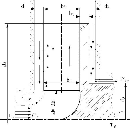
Fig. 1. Scheme of calculations

The equations for the spatial turbulence layer (TL) pulse in the natural coordinates ф and V [2; 3].

We get:

*+R ^(CR) (* - 25" )+ дR   C   дR   x 7

₊ (§• _ 25" = ^T 0 ^a •

R( R    aR) p U2’ дб**   2дб; д( c r ) 1 ,                 .

'+—R—'     '.    б** + б** + б* _ б)+ дR    C    дR    Rx а а /

₊ X /б * _ 2б*Х = _—_ ^Т 0 ^R

R ^{( R    а R} )     R p U²'

If we take the derivatives and perform the necessary reductions, we modify the system (1) to a simpler form:

**

^{д б} а R = ^Т 0а .

д R "p U²’

**

^{д б} R  . ¹ (х** . х* х** 1 —     ^Т0 R

R + R (S. + 6. _ 6R ) = _ и.

Where the characteristic thicknesses of spatial boundary layer are:

– momentum thickness of the longitudinal flow in the direction a

δ

б ;* = J I 1

;

– momentum thickness of the longitudinal flow in the lateral direction

δ

• ** Г I 1 u I ^ю г б_ау? = 1-- —«У ;

^{а R}  0 ( и J и

– momentum thickness of the cross flow in the direction R

5 >2

5 ** Г ^ 7 R =J Vdy .

0 ^U

Here U , ω are the velocities of the longitudinal and cross flows within the limits of boundary-layer thickness δ ; U is the velocity in the flow core on the boundary-layer interface.

The system of differential equations (2) has seven unknown functions in two equations. Making use of the recommendations from [4], we reduce the number of the unknown functions. The expression for the circumferential component of friction stress is the same as the expression for 2-D boundary layer:

= 0,01256 (Re **) ρ U ²

_0,25

**Л ,25                Гт-^

= 0,01256 U^    = 0,01256 c ⁶^

I v J                 I Rv

_ 0,25

where v - is the liquid viscosity; p - is the liquid density; U – is the velocity in the flow core on the BL interface. For the radial component we have t_{0 r} = ет_{0 а} , where £ is the tangent of the angle specifying the direction of bottom streamlines and the wall stress. We introduce the relative significantly positive values

5 **                 C>*                  7-**                  c>*

n        On        On          О

I = -R^-; K = -R-; L = —R-; H = -A

εδ    εδ   ε ² δδ

αααα which are considered to be constant. Let us make substitutions and take the derivatives

_ 0,25

**                       **^**

I б *' ^д^ ■ ^^{д б} '    = 0,01256 C-^

I а дR    дR J I Rv J

**

L 2б ** £ ^^ + £ ² — ^a- + - (8 *‘ + H S ** _ L в ² б **) = I ^а   д R      д R J R^{V а а} ’

**

_0,01256s C5^ I R v

_ 0,25

For the velocity distribution laws in BL of longitudinal U = ( y /6 ) 1^/7 and lateral 6 = 2,12 u ( 1 - u ³) , in accordance with [3] we have H = 1,28; I = 0,46; L = 0,8; K = 2,46. After modifying (4) we obtain the system of two differential equations with two unknowns e and - a* :

- 0'25

• •XC **                  Л_                     ( v-^O** X

  • 0,46ea + 0,465**— = 0,01256e C-^

d R        d R          ( R v J

5 7 **              л_ Q**

0,8e2    a +1,6e5**    + 5 (2,28 - 0,8e2) = dR       a dR   R^’

- 0,25

**

= -0,01256e C-M   ,

I R v J where ε – is the tangent of angle of bottom streamline skewness; -a* - is the momentum thickness in the circumferential direction.

After examining the system of quasi-linear partial differential first-order equations (5) with the aid of the characteristics method [5] we obtain the directions of characteristics of two families coinciding with the angles of their incidence equal to zero. It means that the characteristic of (5) coincides with the coordinate axis R at d/da = 0 . Physically, the momentum thickness - a* cannot be constant, since the static pressure p (force factor connected with variation of pulse with elementary volume) varies along R . It is apparent that the final relation is e = e₀ = const.

Numerous tests for bottom streamline visualization on the surface of canal in wide range of regime and geometrical parameters of LCP have shown that the value of ε varies along the radius and is ctgεcpi

2 C 2 m D 4П _x

U 2 D i

I d2    « , R x arccos ^cos p, „ + —i—

( D 1      ^2л 2 R л

^R 2² 2 R л R i

,

obtained in the case wall facing to the impeller [3]. We have expressed the derivatives in (5) in the explicit form:

- 0,25

ЛО **                  / ^o** X        о**

• —= 0,0703e ^-1 ——     + ' ( 2,853e ^-2 - 1 ) ;

dR            ( R v J     R v          ’ de dR

- 0,25

and replaced the differential relation for ε and pass to the complete differentials:

• - 0,25

**                        ( /-io** X            e**

—= 0,0703e ^{- 1} ——    + ' (2,853e ² - 1). (8)

dR           ( R v J      R           ’

The system (7) can be easily integrated numerically. We note that the initial value of - a* ₀ had been calculated with the use of the technique from [3] in accordance with the principle of BL closure. The results of integrating - a* for three different values of C are presented in fig. 2.

Determining the resistance moment M_{f . w} on the face lateral wall of the canal:

R

M„ = J т 0a 2n R ² dR ,             (9)

where т_{0 а} - is the circumferential component of friction stress determined from (4); R ₂ – is the radius at the impeller outlet; R – is the canal radius. We have modified (8) into the form

M_fw = J 0,01256p ( C/R ²)( C-a Jr v )^{- 0},²⁵ 2nR ² dR ,

R 2

M fw = 0,07892p C '^v⁰,²⁵ J ( - a* / R p²⁵ dR .    (10)

R 2

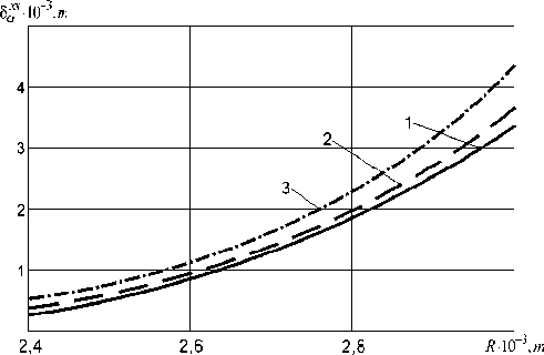
Fig. 2. Distribution of momentum thickness in the circumferential direction for different values of parameter C: 222

1 – C = 1,8      ; 2 – C = 1,2      ; 3 – C = 0,6

sss

The expression (9) is integrated joined with the system (7).

Determining the resistance moment across the cylindrical peripheral part of runner hub M_p we assume that the value of momentum thickness - a* doesn’t vary along the width and is equal to the final value of - a * on the face wall in the radius R . The expression for momentum of resistance on the cylindrical peripheral wall of the canal will then be written

M pw = ^{2n R 2} b ^T 0a ,

M pw = 0,07892p C '^v ^0,25 b ( -“/ R ) 25 , where b – is the canal width.

The experimental data on the resistance moment in the pump canal and the data obtained from (7), (9), (10) coincide with sufficient accuracy which corroborates the validity of the accepted assumptions and the herein presented solution.

We must note that the relations (7), (9), (10) and the solution of the system of equations [2] for liquid rotating over the stationary base in accordance with the solid body law represent in general the closed system of equations for rotor (disk) rotation in closed conditions ensuring the turbulent regime of liquid flow.