On remote sensing of the Earth by spacecraft

Introduction. Remote sensing of a territory is a process which implies collecting information about a territory without direct contact with it [1–6]. In connection with the widespread reduction of the programmes for aerial photography of the earth's surface, satellite imagery of the earth's surface is acquiring special interest. Due to their properties, space images are widely used in both practical and scientific fields [7; 9–11]. Materials of Earth research from space are widely used in Earth sciences. Space imagery is used in research aimed at the comprehensive study of natural resources, the dynamics of natural phenomena, in the tasks of environmental protection. Diverse and widespread use of remote sensing data is especially found in cartography, they serve as sources for the compilation and operational updating of general geographic and thematic maps [8]. Special attention is paid to the use of space information for current operational control over the state of the environment during geoecological monitoring of regions. The main advantages of using remote sensing data for mapping are the following: relevance of data at the time of research, high accuracy in determining the boundaries of objects [12–15]. In particular, this poses the problem in the value of the given parameters at certain points of the earth's surface to find areas of the earth's surface with characteristics determined by the parameters under consideration. In this paper, we consider the special case of this problem when the given four points of the earth's surface determine the regions of the earth's surface (the so-called kernels of generalized squares) that have a specified configuration (square).

Statement of problems, definitions, designations. Mathematical model of the problem. Let a Cartesian coordinate system be given on the plane and A = A ( x A ; у A ) , B = B ( x_B ; y_B ) , C = C ( X c ; y_c ) , D = D ( X d ; y D ) are four different points on the plane, L_A , L_B , L_C , L_D are straight lines passing through the points A , B , C , D respectively. Let us denote by V_AC the point of intersection of the straight lines L_A and L_С , V_AD – the point of intersection

V of the straight lines LA and LD , BC – the point of intersection of the straight lines LB and LС , VBD – the point of intersection of the straight lines LB and LD , VAD; VBD – the distance between the points VAD and VBD , VBC; VBD – the distance between the points VBC and VBD .

The generalized square is a set of lines K A _BCD = { L A , L B , L_C , L_D } with the property that L A is parallel to L_B , L_С is parallel L_D , L_A is perpendicular to L_c , and ( F AD ; V_BD | = | V B _C ; V_BD |. The generalized square kernel is a square with the set of vertices { V AD , V BD , V BC , V AC ^} (fig. 1).

Question 1. Does the generalized square K A _BCD = { L A , L B , L C , L D } always exist at the random selection of the points A = A ( x A ; y A ) , B = B ( x_B ; y_B ) , c = c ( x c ; y c ) , d = d ( x d ; y D ) ?

Question 2. If question 1 is answered negatively, what are the necessary and sufficient conditions for its positive solution?

Question 3. If for the set of the points A = A ( x A ; y A ) , B = B ( X b ; y B ) , C = C ( x c ; y c ) , D = D ( X d ; y D ) the generalized square K A _BCD = { L A , L_B , L_c , L D } exists, how many such generalized squares are there?

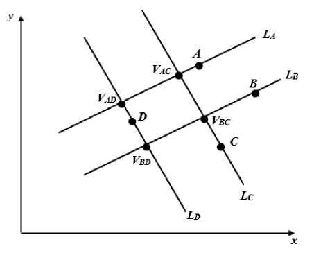
Fig. 1. Generalized square

Рис. 1. Обобщенный квадрат

Partial solution to question 2 and full solution to question 3. In accordance with the above notations, A = A ( ^xA ; y A ) , ^B = ^B ( ^xb ; у в ) , ^c = ^c ( ^xc ; y c ) , D = D ( x_D ; y_D ) are four different points on the plane, L_A , L_B , L_C , L_D – straight lines that pass through the points A , B , C , D respectively. Let us write the equations of these sides according to [16]:

- L A : y = kx + b A - equation of the straight line passing through the point ^A = A ( ^xA ; y A ) ,

- L_B : y = kx + b_B - equation of the straight line passing through the point B = B ( x_B ; y_B ) ,

- Lc : y = -—x + bc - equation of the straight k passing through the point C = C (xc; yc),

- Ld : y = -—x + bD - equation of the straight k passing through the point D = D (xD; yD).

According to the notation introduced above, write down the set of equations for finding line

line

we the

points V_AC , V_BC , V _BD , V_BC and distances    V_AD ; V_BD ,

V_BC ; V_BD .

V AC :

y=kx+b_A ,

- 1

y= x+bC, k where bA =yA

^- kx_A ^,bc = y c+-^xc . k

V AC :

V AC =

V BC :

У = ^kx + ( У а ^{- kx}A ) ,

У = ^-7 ^{x +} l У с +7 x c I , k I k )

( k2 ( yC - yD ) + k ( xC - xD )) +

x =

У =

k 2 xA + k ( Ус - Уа ) + xc

1 + k k2yc +k(xc -

,

1 + k ²

;

y = kx + bB, y = -- x + bc, k

x =

k ² x_B + k ( y_c - y_B ) + x_c

V BC =

1 + k²

,

У =

( x c

1 + k ²

;

V AD :

’ У = ^kx + b A ,

1 , y = - x + bD , I k

x =

^k 2 x A + ^k ( y D ^- У a ) + x D ,

V AD =

V BD :

У =

1 + k ^{k 2} y D + к ( x_D-

+ (k(Ус - yD) + (xc - xD ))2 2.

Squaring both sides of the above equation, we obtain: ^k 4 ^{( x}A ^{- x}B ) ^{+ 2 k} 3 ^{( x}A ^{- x}B ^{)( y}B ^{- y}A ^{) + k 2 ( y}B ^{- y}A ) ^{+ + k 2 ( x}B ^- x A ) ^{+ 2 k (} x B ^- x A ^{)( y}A ^{- y}B ^{) + ( y}A ^{- y}B ) =

= k4 (yC - yD ) + 2k3 (yC - yD )(xC - xD ) ++ k 2 (xC - xD ) + k 2 ( yC - yD ) +

+ 2k(Ус -yD)(xc -xD) + (xc -xD)2-

After reducing the similar terms with respect to k, we obtain the biquadratic equation:

^{k 4} [ ( ^xA ^{- x}B ) ² - ( У с ^- y D ) ² ] ⁺

k3 [2(xA - xB )(yB - yA) - 2(yC - yD )(xC - xD ))] + k 2 [( yB - yA ) +( xB - xA ) -( xC - xD ) -( yC - yD ) ] + k[2(xB -xA)(Уа - Ув )- 2(Ус -yD)(xc -xD)] +

1 + k ²

^xA ) ⁺ Уа .

;

^[( У а ^- У в ) 2 ^-( ^xc ^{- x}D ) 2 ] = 0-

Dividing both sides of this equation by the coefficient at k ⁴, we obtain the following equation:

y = kx + bB, y = -- x + bD , k

k ⁴ + k ³

² ( ^xA ^{- x}B ) ( У в ^- У а ) ^{- 2} ( У с ^- y D )( ^xc ^{- x}D ) ) ( x A ^- x B ) 2 ^-( У с ^- y D ) 2

V BD =

x =

^{k 2 x}B + ^k ( y D ^- У в ) + x D

y =

1 + k ^{k 2} y D + k ( XD"

1 + k ²

k ²

I V AD ;V BD | = ^{( k 2 (}

^xB ) ⁺ Ув . ^;

xA - xB) + k(Ув - Уа ))2 +

+ (k (xB - xA) + (Уа - Ув ))2

∙

1 + k ²

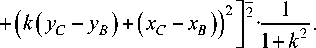
I VBC ; ^ BD | =

(k2 (Ус - yD) + k (xc - xD)) +

+ (k (yc - yD) + (xc - xD ))2

1 + k ^2.

Since the sides of the square are equal, we search for k from the condition | V_AD ; V_BD |=| V_BC ; V_BD |:

( k 2 ( xA - xB ) + k ( yB - yA )) +

+ (k (xB - xA) + (Уа - Ув ))2 2 =

( yB - yA ) +( xB - xA ) -( xC - xD ) -( yC - yD )

( x A ^- x B ) 2 ^-( У с ^- y D ) 2              .

+

k

2(xB - xA)(Уа - Ув )- 2(Ус - yD)(xc - xD)

( x A ^- x B ) 2 ^-( У с ^- y D ) 2           .

(Уа - Ув )2 -(xc - xD )2

( x A ^- x B ) 2 ^-( У с ^- y D ) 2

= 0.

This yields the partial solution to question 2 and the full solution to question 3.

Partial solution to question 2 (sufficient condition for the existence of a generalized square). To make the equation have a real root, it is sufficient to satisfy the inequality:

( Уа - Ув )2 -(xc - xD )2(xA - xB )2 -( Ус - yD )2

< 0.

Solution to question 3. According to [17], this equation has no more than 4 different real roots. Since with the considered situation we can consider a certain case L A is parallel to L_C and a certain case L_A is parallel to L_D, then the total number of generalized squares for a fixed set of points A = A ( x a ; У а ) , B = B ( x b ; У в ) , C = C ( x c ; У с ) , D = D ( x_D ; y_D ) is no more than 12. It is obvious that the estimate is accurate.

Case Study. As our example we take the following: A ( x A ; у а ) = ( 5;6 ) , B ( x B ; У в ) = ( 7;5 ) , C ( x c ; У c ) = ( 4;3 ) , D ( x_D ; У_D ) = ( 3;4 ) and we consider three different situations.

1. L_A is parallel to L_B

After substituting the coordinates of the given points into the formula (8), we obtain the equation

3 k ⁴ + 6 k ³ + 3 k ² + 6 k = 0.

VBC

We find the roots of this equation: k 1 = 0, k ₂ = - 2, k 3 = i , k ₄ = - i , wherei ² = - 1.

We calculate the coordinates of the vertices of the generalized square for the root k = k 1 = 0 using the formulae:

k ² x_A + k ( y_c

^^^^^^B

V Ac =

У =

1 + k k ² y_c + k ( x_c -

Уа ) + xc

,

V AD

^^^^^^B

1 + k ²

XA) + Уа

,

V AC ^{( X}C ; y A ) = V AC ^{( 4;6 )} ,

k2xb +k(yc x =-----—

^^^^^^B

V Bc =

У =

1 + k k ² y_c + k ( x_c -

Ув) + xc

,

^^^^^^B

1 + k ²

xв) + Ув

,

^Vвc ^{( x}c ^{; у}в ) = ^vbc ^{( 4;5 )} , _x = ^{k 2 X}A ⁺ k ( У D

^^^^^^B

V AD =

У =

1 + k ^k 2 y D ^{+ k} ( ^XD

Уа ) + xd

,

V BD

^^^^^^B

1 + k ²

xa ) + Уа

,

V AD ^{( X}D ; y A ) = V AD ^{( 3;6 )} ,

x

y

x

y

x

y

k 2 xв + k ( yc - Ув ) + xc
1 + k 2
( - 2 ) 2 7 + ( - 2 )( 3 - 5 ) + 4	36
1 + ( - 2 ) 2	5,
k 2 yc + k ( xc - xв ) + Ув
1 + k2
( - 2 ) 2 3 + ( - 2 )( 4 - 7 ) + 5 _	23
1 + ( - 2 ) 2	5,
k 2 XA + k ( У D - У A ) + XD
1 + k 2
( - 2 ) 2 5 + ( - 2 )( 4 - 6 ) + 3	27
1 + ( - 2 ) 2	5
k 2 У D + k ( XD - XA ) + У A
1 + k 2
( - 2 ) 2 4 + ( - 2 )( 3 - 5 ) + 6	26
1 + ( - 2 ) 2	5
= k 2 xв + k ( У D - У в ) + XD
1 + k 2
( - 2 ) 2 7 + ( - 2 )( 4 - 5 ) + 3 =	33
1 + (- 2 ) 2	5
, = k 2 У D + k ( XD - XB ) + У в
1 + k 2
( - 2 ) 24 + ( - 2 )( 3 - 7 ) + 5 _	29
1 + ( - 2 ) 2	5

V вD ( 6.6;5.8 ) .

,

,

,

,

,

,

V ad ( 5.4;5.2 ) ;

V вc ( 7.2; 4.6 ) ;

V BD =

x = ^k 2 ^XB ^{+ k} ( y D

^^^^^^B

У =

1 + k k2yD +k(XD

Ув ) + XD

,

^^^^^^B

1 + k ²

xв) + Ув

,

V BD ^{( x}d ^{; y}B ) = V BD ^{( 3;5 )} .

Direct calculation shows that

I V ; ] =1 V ; V 1 = V AC BC BC BD B

BD ;

^; VAD |=| VAD ^; VAc | = ¹ •

It follows that the quadrangle with the vertices V_AD , V_BD , V_BC , V_AC is a square (fig. 2).

We calculate the coordinates of the vertices of the generalized square for the root k = k ₂= –2 using the formulae:

x = k 2 XA + k (Уc - Уа ) + xc = x 1+k2

_ ( - 2 ) 2 5 + ( - 2 )( 3 - 6 ) + 4 _30

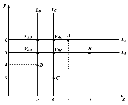
Fig. 2. Generalized square for the root k 1 = 0

V AC

1 + ( - 2 ) 2

У =

k ² y_c + k ( x_c

^^^^^^B

XA ) + Уа =

V ac ( 6;4 ) ;

Рис. 2. Обобщенный квадрат для корня k ₁ = 0

1 + k ²

_ ( - 2 ) 2 3 + ( - 2 )( 4 - 5 ) + 6 _20

1 + ( - 2 ) 2

Direct calculation shows that

⁰ | ^VAD ; ^BD |=| ^VBD ; V Sc ] = | ^VBC ; V Ac |=| V Ac ; V AD | = 5Ц ■

It follows that the quadrangle with the vertices V_AD , V_BD , V_BC , V_AC is a square (fig. 3).

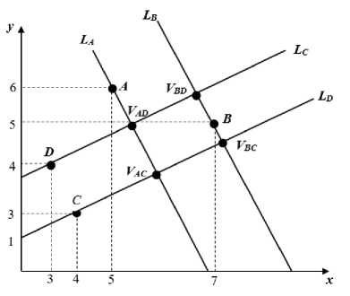
Fig. 3. Generalized square for the root k 2 = –2

V AD :

y = kx + b A ,

1 y = -- x + bD, k x = k 2 xA + k ( yD

V AD =

V CD :

^^^^^^B

Рис. 3. Обобщенный квадрат для корня k ₂ = –2

2. The straight line L A is parallel to the straight line L C

The general equations of required sides in this case are the following:

L A : y = kx + b A - equation of the straight line passing through the point A ( x A ; y A ) ;

LB : y = -1 x + bB - equation of the straight line pass-k ing through the point B (xB; yB);

L C : y = kx + b C - equation of the straight line passing through the point C ( x C ; y C ) ;

Ld : y = -1 x + bD - equation of the straight line pass-k ing through the point D (xD; yD).

Let us write down the set of equations for finding the vertices of the square in this case:

f y = kx + b A ,

V AB : i     - I

I y = —^{x + b}B , I      k

where ^bA =y A ^- kx A ,b B = У в + 1 x B ; k

У = ^{kx +} ( У A ^- kx A ) ,

У = -T ^x + У в ⁺ Tx B k I k

x =

k 2 xA + k ( Ув - yA) + xB

У =

1 + k k 2 yD +k(xD

yA ) + xD

,

^^^^^^B

1 + k ²

y = kx + bc, y = -- x + bD , k

k ² x C + k ( y_D x =------—

^^^^^^B

V CD =

У =

1 + k k2yD +k(xD-

V AB =

y =

1 + k ²

^k 2 У в ^{+ k} ( ^xB ^{- x}A ) ⁺ У A

1 + k ²

V BC :

y = kx + b C ,

У = -- x + bB, k

V BC =

x =

У =

k ² x C + k ( y_B - y C ) + x_B 1 + k ²

k 2 y_B + k ( x_B - x C ) + y C 1 + k ²

xA) + yA

.

yC) + xD

,

^^^^^^B

1 + k ²

.

xC ) + yD

.

After substituting the coordinates of the points into the formula, we obtain the equation

2 k ³ + k ² + 2 k + 1 = 0.

We find the roots of this equation 1

k 1 =- 2, k ₂ =- i ,k ₃ = i , where i =- 1. We calculate the coordinates of the vertices of the generalized square for a real root k = k 1 = - 2 according to the formulae pre-

sented above.

x = ^{k 2 x}A ^{+ k} ( У в

- yA) + xB

1 + k ²

V AB

V BC

1Y ^^^^^^B

2 J

У =

5 - 2 ( 5 - 6 ) + 7

1 ( 1 ) 2

1 + -

I 2 J

^{k 2} У в ^{+ k} ( ^xB

^^^^^^B

1 + k ²

1 ( 1 1 2

1 + -

I 2 J

k ² x C + k ( y_B x =------—

1Y ^^^^^^B               I

2 J

У =

= 7,

xA) + yA =

V AB ( 7;5 ) .

= 5,

- yC) + xB

1 + k²

4 - 2 ( 5 - 3 ) + 7

1 ( 1 )2

1 + -

I 2 J

k 2 У в + k ( x b

^^^^^^B

1 + k ²

1 ( 1 1 2

1 + -

I 2 J

5,

^xC ) ⁺ y C _

V bc ( 5.6;2.2 ) .

5,

vad _ *

V CD

x _ ^{k 2 x}A ^{+ k} ( y D

- yA ) + xD

¹1 2 ^^^^^^B

2 J

У _

1 + k²

5 - 2 ( 4 - 6 ) + 3

1 ( 1 1 2

1 + -

I 2 J

^{k 2} y D ^{+ k} ( x D

^^^^^^B

2 J

^^^^^^в

5,

x A ) + У а _

1 + k ²

^{4 -} 2 ( 3 ^- 5 ) + 6

1 ( 1 1 2

1 + -

I 2 J

k ² x_C + k ( y_D

^^^^^^B

2 J

У _

V ad ( 4.2;6.4 ) .

5,

- y c ^ + x D

1 + k ²

4 - 2(4 - 3)+3

1 f 1 )2

1 + -

I 2 J

^{k 2} y D ^{+ k} ( ^xd

^^^^^^B

5;

^xC ) + y D _

V cd ( 2.8;3.6 ) .

¹ 1 2 ^^^^^^B

2 J

1 + k ²

^{4 -} 2 ( 3 ^- 4 ) + 3

1 f 1 1 2

1 + -

I 2 J

5;

Direct calculation shows that

|VAB ; ^BC |^_| VB

BC ;

; V DC I ^_ I V AD ; V DC |^_| V A

AD ;

.

Consequently, the quadrangle with

V_AB , V_DC , V_BC , V_AD is a square (fig. 4).

the vertices

Fig. 4. Generalized square for the root k = –1/2

Рис. 4. Обобщенный квадрат для корня k = –1/2

3. The straight line L A is parallel to the straight line L D

Let us write down the general equations of required sides in case when the straight line L A is parallel to the straight line L D , in this instance:

L A : y _ kx + b_A - equation of the straight line passing through the point A ( x_A ; y_A ) ;

LB : y _-1 x + bB - equation of the straight line pass-k ing through the point B (xB; yB);

Lc : y _ -1 x + bc - equation of the straight line pass-k ing through the point C (xC; yC);

L D : y _ kx + b_D - equation of the straight line passing through the point D ( x_D ; y_D ) .

The system of equations for finding the vertices of a square in this case is written as follows:

) y = ^{kx + b}A ,

where b_A =y_A

V AC

V AC

VDC

V DC

V BD

VBD

V AC ^: *     ^{- 1}

I ^y = T ^{s + b}C ,

- kxA,bC =yC+TxC . k y _ kx + ( Уа - kxA ), : *            1 . f .1 1

у ^_-T ^{x +} l y C ⁺t ^xc I , k I k )

k ² x_A + k ( y_C x _------—

У _

^^^^^^B

1 + k k ² y_C + k ( x_C -

Уа ) + xC

,

^^^^^^B

1 + k ²

y _ kx + bD, y _--x + bC, k

_ *

_ *

x A ) + У а

.

k ² x_D + k ( y_C x ^_          1 + k²

y _

k ² y_C + k ( x_C

^^^^^^B

yD ) + xC

,

^^^^^^B

xD ) + yD

1 + k ²

.

y _ kx + b_D

1, y _--x + bB k

_ k 2 xD + k ( Ув - yD ) + xB x —              9

1 + k ²

_ k2 Ув + k ( xb - xd ) + yD y           1 + k2

.

Let us find the distance between the points.

I V AB ; ^VDb \ ^_ ( k ^{2 (}

+ ( k ( xD

^^^^^^B

xA

^^^^^^B

xD) + k (yD - Уа )) +

xA ) + (У A - yD ))2

•------—

1 + k ².

I ^Vdc ^{; V} db | = l ( ^{k (} y c   ^yB ) ^{+ k (} x c   ^xB ) ) ⁺

Let us define k from the condition

| VAB ; ^ DB ¹=| ^ DC ; ^ DB |

VDC = '

(к2 (Xa - Xd ) + k (yD - Уа ))2 +

+ (k(xD - Xa ) + (Уа - Vd ))2 2 =

k ² x_D + k ( y_c - y_D ) + x_c

=         1 + k2

( - 0.28) 2 3+I _Z 0.28) ( 3-4)₁4 = 4 51;

1 + (-0,28)2. ’ k2 yc + k (xc - xD) + yD y =----W

(-0.28)23+j-0.28)^4-3) + 4 = 3 66;

1 + (-0.28)2. ’

V_DC ( 4.51;3.66 ) .

(k2 ( Ус - Ув ) + k (xc - Xb )) +

+ (k(Ус - Ув ) + (xc - Xb ))2 2

VAB = "

x =

k 2 Xa + k ( Ув - Уа ) + Xb =

1 + k k -

= ( - 0.28 ) 2 5 + ( - 0.28 )( 5 - 6 ) + 7

Let us square both sides of the resulting equality:

^k 4 ( ^Xa ^{- X}d ) 2 ^{+ 2 k} 3 ( ^Xa ^{- X}d )( V d ^- У а ) ⁺

+ k2 (yD - yA ) + k2 (XD - XA ) + 2k(XD - XA )(yA - yD ) + +(Уа - Vd)2 = k4 (Ус - Ув )2 + 2k3 (Ус - Ув )(xc -Xb ) + + k 2(xc - Xb ) + k 2(yc - yB) +

1 + ( - 0.28 ) 2

= k 2 Ув + k ( Xb - Xa ) + Уа y           1 + kг

= (-0.28)2 5 + (-0.28)( 7 - 5) + 6

V ab ( 7.1;5.4 ) .

= 7.1;

1 + ( - 0.28 ) 2

= 5.4;

+ 2k(yc -yB)(xc -Xb) + (xc -Xb) •

After reducing the terms in regard to the power of k of additive components, we obtain the following equation:

k4 [(Xa - Xd)2-(Ус -Ув)2] +

+ k3 [2(Xa - Xd )(Vd - Уа) - 2(Ус - Ув )(xc - Xb ))] + +k 2 [(yD - yA ) +( XD - XA ) -( xC - XB ) -( yC - yB ) ] + +k[2(Xd - Xa )(Уа - Vd )-2(Ус -Ув )(xc -Xb )] = 0.

We substitute the coordinates of the points into the equation and we obtain the equation with numerical coefficients:

20 k ³ + 12 k ² + 20 k + 5 = 0.

We find the roots of this equation k 1 =- 0,28, k ₂ = 0,16 + 0,94 i , k ₃ = 0,16 - 0,94 i .

We calculate the coordinates of the vertices of the

VBD = '

generalized square for a real root k = k 1 = - 0,28 accord-

ing to the formulae presented above:

k 2 Xa + k ( Ус - Уа ) + xc

1 + k²

( - 0.28 )2 5 + ( - 0.28 )( 3 - 6 ) + 4

x =

k 2 Xd + k ( Ув - Vd ) + Xb _

1 + k^г

_ ( - 0.28 ) 2 3 + ( - 0.28 )( 5 - 4 ) + 7

1 + ( - 0.28 ) 2

= ^{k 2 y} B ^{+ k} ( ^Xb ^- y”          1 + k^г

= 6.4;

^Xd ) ⁺ V d _

_ ( - 0.28 ) 2 5 + ( - 0.28 )( 7 - 3 ) + 4

V bd ( 6.4;3.96 ) .

V ac =^

y =

1 + ( - 0.28 ) ^k 2 У с ^{+ k} ( x c

^^^^^B

1 + k²

= 4.85;

^Xa )⁺ У а =

( - 0,28 )2 3 + ( - 0,28 )( 4 - 5 ) + 6

1 + ( - 0,28 )2

= 6,08;

1 + ( - 0.28 ) 2

= 3.96;

Direct calculation shows that

| VAC ^{; V} DC |=l ^V AC ^{; V} Ba| = | ^V BD ; ^V DC |=| ^V BA ; ^V BD | = ^2.25

Consequently, the quadrangle with the vertices V_AC , V_DC , V_BA , V_BD is a square.

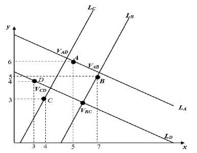
Fig. 5. Generalized square for the root k = –0.28

V ac ( 4.85;6.08 ) .

Рис. 5. Обобщенный квадрат для корня k = –0,28

Thus, for a given set of points, there are 4 generalized squares shown in fig. 2–5.

Conclusion. Remote sensing by spacecraft is a rapidly developing technology-based field. One of the most important components ensuring this development is the mathematical apparatus underlying the operation of the algorithms incorporated into the operation of spacecraft and providing the required parameters for sensing the earth's surface. The problem being considered in this work is devoted to this issue.

Sensing algorithms built on its basis will effectively obtain information about the state and boundaries of individual sections of the earth's surface within a short time (depending on the values of a finite number of specified parameters). The method being considered can naturally be expanded by changing the conditions imposed on the form of lines (not necessarily straight) passing through selected points on the earth's surface and intersecting under the conditions that are different from those given in the work under consideration.