On the computation and applications of bessel functions with pure imaginary indices (orders) in physics and specifically in corpuscular optics

Bessel functions occur in many branches of mathematical physics [1, 2, 12, 13] as solutions to differential equations when the Dirichlet and Neumann boundary conditions are applied on various space domains such as cylindrical or spherical. In a great variety of these applications (diffraction, electrical induction, etc.) only Bessel functions of the zeroth and first orders namely J 0 ( x ) and J 1 ( x ) occur. In other physical applications (such as solutions to Kepler’s equation), the entire index n of J_n ( x j are used. The Bessel functions of complex-valued indexes have had limited number of applications up till now. Presently (to the best of our knowledge) there is no existing mathematical software package or algorithm that computes these functions in their entire domain of definition as they have not been found applicable in areas of physics. The normal and modified Bessel function of pure Imaginary order was shown to be the solution governing the motion of corpuscular particles in isotrajectory focusing and deflecting systems [3]. Recently it was shown that they also appear as solutions to the Lame’s equation which are used to characterize the displacement fields in semiconductor nanostructures. Usually the Bessel function of pure imaginary order with real or complex valued argument is defined with the aid of the complex Gamma function [4]. Obtaining the real values of these functions, however, is very vital in mathematical physics and applied sciences. The Bessel functions of order v can be represented as the solutions to the following differential equation [5]:

x ² y" + xy ' + ( x ² - v ² j y = 0,           (1)

where y' represent the first derivative with respect to x .

The resulted function can be expressed as an absolute converging series iv                       (yX

I § ( - 1 ) n r v + n + 1j 1 2 J

Even though the above function has whole number values of ν in the entire complex plane, it is practically non-trivial to compute this function for non real values of the index. Most computations and computational packages nowadays on this basis require that each element of the series is obtained via a complex Gamma function [4]. For instance for the case of a purely imaginary index i ν and for a natural number n , we have

r ( i v + n + 1 j = F ( i v j^ n [ ( i v + m j . (3) m = 0

Hence to compute real solutions for equation (1) for purely imaginary order, it is required to sum a series with each coefficient being a complex number and not to forget the case of obtaining the complex value function r ( i v j , which on its own is very cumbersome to compute. Also to the best of our knowledge, there is no concrete algorithm that computes Bessel functions with pure imaginary order despite the fact that they were discovered decade ago.

The author of one of the vastest treatment of Bessel functions [5] thought that these functions had no great interest. However these functions were noticed by Lommel [6] and he defined the function J _{v + i} . ( z ) :

. .             (x)2)v+i"

J ( z ) =X ^{v +1Л} ’ r ( /2 ) r ( v + i . + 1/2 )

x[Kv,. (x) + ^ (x)] ,

with K and S being real valued functions. This representation by Lommel, however, does not make the computation of these functions any easier. Lommel attempted to obtain a computable integral representation of the Bessel functions to no avail. He however derived the following differential equation as a motivation for the solutions:

x ² y" + ( 2 a - 2 ev + 1 ) xy' +

+ [a(a - 2ev) + в Y2 x 2e ]• У = 0,(5)

this equation has solution (for real nonzero β ) which can be written in the form y = xev-a [AJv (Yxe) + BJ-v (Yxe)].(6)

Comparing equation (5) above with the equation x2 y" + axy' + (b + cx2 e) y = 0,(7)

it can be shown [6] that the coefficients in equation (5) and equation (6) have relations shown below ev - a = -( a -1)/2,(8)

ev = [(a -1)/2]2 - b, ev = Tc .(9)

It showed that the real valued coefficients ( a , b , c ) gave in general case solution as equation (6) with complex index ν . This was also identical to that suggested [3] as possible solution with complex index. At the end, Lommel obtained a very cumbersome solution to equation (7), with real valued coefficients as multiples of a complex valued function. However, no mechanism for the computation of its real valued solution was proposed or mentioned.

Another mathematician M. Bocher approached the modified Bessel function with pure imaginary index while he proposed solutions to Laplace’s equation by method of variable separation in cylindrical coordinates [7]. It is very important role of Bessel function with pure imaginary index in mathematical physics.

As opposed to [6], Bocher proposed real valued solutions with the aid of real valued series (however, the convergence of these series was never studied). Each of the coefficients in the series solution suggested in

[7] was partially a polynomial function in ν that grew as n !). This approach was found to be intuitive [7]; however, it needed large numbers of iterations as the terms in the series grew. This gave a major problem for its convergence.

Finally the McDonald’s function K _{i T} ( x ) with pure imaginary index was used in the integral representation to solve Laplace and wave equations with different boundary values [8]. The author [8] used the representation to

' K _{i t} ( x ) = j exp ( - x cosh t ) cos ( Tt ) d t , x >  0.     (10)

The representation above was found to be valid only for sufficiently large values of the argument x . Unfortunately for small values of x this integral representation is not effective, where pure imaginary indices Bessel functions become applicable and useful in electron optics dynamics [3] and strain field investigations in nanostructures.

The above summary shows that there is not yet an effective algorithm for the computation of Bessel functions with pure imaginary indices.

METHODS AND CALCULATIONS

George Boole [9] developed an operation method to solve differential equation over a century ago. This approach considered calculus as is the treatment of symbols that stands for the operations (e. g., taking the derivative of a function) as if they stood for numerical quantities. Based on the intuition from [9] we can consider the solutions to the equation (1) to be expressed in form y = A (x) cos (v ln x) + B (x) sin (v ln x), (11) where A (x) and B (x) are series with the coefficients as shown:

A ( x ) = a 0 + a 1 x + a ₂ x ² + • • • a n x" + — , B ( x ) = b ₀ + b j x + b ₂ x ² + • b n x " + •

Substituting equation (11) into equation (1) and equating the zeros of the coefficients before the linearly independent functions cos (v ln x) and sin (v ln x), we obtain firstly the relation, a1 = b1 = 0,                    (13)

and secondly Vn > 2 the recurrent relationship na"-2 - 2vb"-2

n ( n ² + 4 v ²) ,

b n =

^{2 v} a n - 2 + ⁿ b n - 2 n ( n ² + 4 v ²)

M 2 n ^

From equation (14) and (15), it is clearly seen that odd term coefficients are identical to zeros while those with even values can be obtained via a recurrent relation using the values a ₀ , b ₀ . The series solution to the Bessel equation (1) was first introduced by Boole [9], however, he failed to provide analysis regarding the convergence of the series.

The Boole’s recurrent relation thus had to be modified to serve our needs. They can also be readily computed since they seem to exist only for even indices. Let us re-define the function A ( x ) , B ( x ) such that

1             v

_    + Г 2A M 2 n - 2

n + v   n ( n + v )

" 72 + v ¹ M

V ^{n n} J

2 n - 2 .

The inequality (20) allows us to be able to test and study the rate and order of which the majorant M _{2 n} decays and it is trivial to show that it obeys:

ν

^M 2 n ^ C— , ⁽ n ^{! )}

”        2 n

A(x) = ^a2n22nI-I n=0        V 2 J

~     2rYⁿ

= Z A 2 n к I ,     (16)

n = 0      V ² J

”         (² n

B(x ) = 7b 2^{2 n} I x I

2n n=0        V 2 J

~     2rYⁿ

=     B ₂ I I

2n I I n=0 V 2 J

.

Now for n >  1 the coefficients A 2 _n , B _{2 n} can be reduced to

A

nA 2 n - 2   ^VB 2 n - 2

n ( n ² + v ² )

B, =

2 n

^vA 2 n - 2 ⁺ n ^B 2 n - 2 n ( n ² + v ² )

where C is a positive constant defining the zero term of the sequence. Using the d'Alembert's test for convergence [11] the proof of absolute convergence for all values of x and ν is completed. We can now without lost of generality form two linearly independent solutions for (1).

Let us choose two pairs of the values for A ₀ , B ₀ that are generated from the sequences A _{2 n} , B _{2 n} with corresponding functions defined by (16) and (17). Under these conditions there exist two solutions for (1). Based on the rate of convergence of the majorant (22), the linearly independent solutions to (1) are shown to be easily computable with algorithm that contains a very limited number of iterations. The solution spawned from the pair

( A 0 , B 0 ) = ( 0,1 ) , (23)

PROOF OF CONVERGENCE AND CONSTRUCTION OF COMPUTABLE SOLUTIONS

was notated in [3] as Sf _v ( x ) and Cf _v ( x ) as that spawned from the pair

( A ,, B о ) = ( 1,0 ) ,                  (24)

In order to compute the strain fields in nanostructures or to implement the Bessel function in other areas of physics, we need to be able to show that the solutions to this differential equation exist and most of all converges in our domain of interest. We now show that the series (14, 15) converges and does so absolutely for any complex value argument and with any value of the order v . According to [10, 11], a series will converge absolutely if and only if the absolute value of the n -th term (which shall be referred to as the majorant) converges. Let the majorant M _{2 n} be defined such that

M 2 n = | A 2 n | + B 2 n | , (20)

then we can easily obtain the analytical expression of these new functions

Sf v ( x ) = 1

—

1    I x I ²

1 + v² V 2 J

+ ••• sin ( v In x ) +

from (18), (19) and (20) it can follow that

+

v

1 + v²

Cf v ( x ) = 1

—

+

v

1 + v²

1    I x I ²

1 + v ² V 2 J

+ ... cos ( v In x ) +

For small values of the argument x ^ 0, we have two equivalent relationships

Cf v ( x ) ~ cos ( v In x ) ,           (27)

Sf_v ( x ) ~ sin ( v In x ) .            (28)

Hence we see that the symbol used to define this new function are also linked by the equivalent relation and clearly defines physical models earlier proposed [3] and strain field characterization for some nanostructures. Now the general solution of the differential equation (1) can be explicitly written out in the form

y = c Sf v ( x ) + c ₂ Cf v ( x ) .         (30)

This solution also allows us to easily construct real valued solutions and functions for the modified Bessel function with pure imaginary index, i.e. to solve the equation

for (31). Now we can construct two linearly independent solutions for this case. We observe that by choosing two pairs of values C0,D0 obtained from their respective series expressions, we can easily construct two real valued functions being solutions y1 = C (x) cos (vlnx) + D (x) sin (vlnx), (38)

y ₂ = D ( x ) cos ( v ln x ) - C ( x ) sin ( v ln x ) . (39)

It is clear that to form two linearly independent solutions to (31) it suffices to take one pair of the spawned sequence

( C 0 , D 0 ) = ( 0,1 )

x ² y " + xy ' + ( - x ² + v ² ) y = 0.        (31)

substituting (34) and (35) into (38) and (39), we ob tain two functions denoted [3] as

Sd_v ( x ) and Cd_v ( x ) :

cos ( v In ix ) = cosh

-

Sd v ( x ) =

1 +

1 + v v

+ •••

sin ( v ln x ) +

- sinh — sin ( v In x

( 2 J ^V

+

v f x 1

+•••

1 + v2 uj

cos ( v ln x ) ,

sin ( v In ix ) = cosh f ^ 1 sin ( v In x ) +

Cd v ( x ) = 1 +

1 + v v

-

, ■ , ( nv 1 z z + sinh — cos ( v In x ) ,

I 2 J

-

-

where sinh and cosh are the hyperbolic sinus and cosine functions respectively. We can also define functions C ( x ) , D ( x )

v

1 + v v

for small values of the argument x ^ 0, we also have

Cd

C (x ) = A (ix ) = £ C2i n=0

2 n

two equivalent relationships

Cd_v ( x ) ~ cos ( v ln x ) , Sd_v ( x ) ~ sin ( v ln x ) ,

d

D ( ^x ) = B ( i x ) = E D 2.

n = 0

And as in the earlier section, for n >  1 the recurrent equation for C _{2 n} , D _{2 n} takes the expected form

^C 2 n ⁼

^nC 2 n - 2   ^vD 2 n - 2

n ( n ² + V ² )

I = vC2 n-2 + nD2 n-2 2 n           / 2      2 \ n (n2 + V 2)

And it is very trivial to show that (36) and (37) converges absolutely for any x and v . One real valued solution for (1) spawns two real valued solutions

(43) and (44) shows again that these functions are linearly independent and also solutions to (31).

ALGORITHM FOR THE COMPUTATION OF FUNCTION

Cd v ( x ) , Sd v ( x ) , Cf v ( x ) , Sf v ( x )

An important property that has to be analyzed for easy computation of these functions is the Wronskian. In mathematics, the Wronskian is a function named after the Polish mathematician Józef Hoene-Wroński., where it can be used to determine whether a set of solutions are linearly independent [12, 13]. It can be easily shown that the Wronskian W of two linearly independent solutions of the equation y" + Xy ‘ + f (x) y = 0,         (45)

has the form W = a, with the constant a depending x on the concrete solution. The equivalent relationship (27), (28) and (43), (44) allows us to be able to obtain a

Cf v ( x ) [ Sf v ( x ) ]‘ - Sf v ( x ) [ Cf v ( x ) ]‘ = X,      (46)

Cd v ( x ) [ Sd v ( x ) ]' - Sd v ( x ) [ Cd v ( x ) ]' = x.    (47)

It clearly shows that the Wronskian (46) and (47) vanishes for v = 0. Leading to the following relationship v ^ 0 ^ Cfv (x )^ Jо (x),

Sf v ( x ) ^ 0.

Choosing more terms of the Taylor’s series, we can further give the possibility of increasing the accuracy

-mn -— 1 ++ .

m         n2

2 n - 2

Taking the natural logarithm of both sides of (50), we obtain:

v2 Fv ln ( m2n ) - ln ( m2n-2 ) < ln(1 + — + —) < ~ nn n

Using the well known sums below, ю^2

x 4=-1, n^2 n2

F

⁺    3 .

n ³

jr -13 = Z(3) -1 = 0.2021, n=2 n and also the value for

ACCURACY OF COMPUTATIONAL ALGORITHM

m 0 = 1,

To obtain a measure of the computational error, we required a detailed study of the majorant (remainder) M _{2 n} . To understand this, let us consider the following series

finally, we obtain

m ₂ =

1 ± M

1 + v 2 ,

nv

M 2 n = —2 m 2 n .

⁽ n ^{! )}

with

Now we obtain an estimate for remainder m _{2 n} for n >  2

m _{2 n}

( 1 + И 1

v

m 2 n - 2

< n J

n

Using Lagrange’s formula for remainders, the Taylor’s series [10, 11] gives for n >  2

^m 2 n ^i ^{v 2} . I ^v l ⁽I v l - 1K ⁹ ^ v - 2 — 1+1

m         n ²     6 n ³        n

2 n - 2

where 0 — 9 — 1.

We can thus reduce the inequality (49) by removing from the right hand side θ

m2n      v2   F m 2 n-2      n    n

ln-m2^ < 0.6449v2 + 0.2021F m 2 n-2

1 + v             2

m _{2 n} < —Ц exp(0.6449 v ² + 0.2021 F ) = m .

^{2 n} 1 + v ²

Now, the accuracy for М 2n takes the form

v

M ₂ „< m---т            (53)

^{2 n}       ( n !)²

We can conclude by saying that the sum of the remaining terms for the series functions

A ( x ) , B ( x ) , C ( x ) , D ( x ) cannot exceed the value

to

£ = m £ n=N

n^v ( n !)²

Since the remainder will depend on the value of v,

we thus study the case | v | — 2 , then

2 m

^£ n ^— m T £

⁴ n = N + 1

2 n - 2

x )

[ ( n - 1 ) ! ] 2 ( 2

V2 ”    1           n xx

= m

4 ^£ ( n !)² ( 2 ¹

.

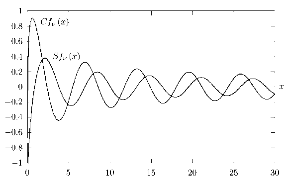
Fig. 1. Functions Sf _/2 ( x ) and Cf y₂ ( x ) for 0 <  x <  30

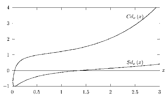
Fig. 2. Functions Sd 1,2 ( x ) and Cd ₁₍₂ ( x ) for 0 <  x <  3

The sum at the RHS of this series is simply the remainder of the series for the modified Bessel function of zero 1 ₀ ( x ) . This remainder can also be evaluated further as shows below

1 I x

X

( N ! ) ² 1 2

2 N + 1

”

n = N ( n ! )

Eliminating v we obtain estimates for х and v

( ^N ! ) ²

x I ² N ^,    ( N ! ) ²

² J n = 0 [ ( n + N ) ! ]

2 N + 1

^ <  15         -     I. ( x ) .

^N      ( N ! ) ² 1 2 J ^{1 (} )

Partial for x <  2 , the equation above reduces to

1   | x I N <

( N ! ) 2 1 ² J "

1      1     ( x Y

1 +             +•••+

( 1 + N ) 2 1 2 J

N " ( N ! ) 2 ^.

2n x I

2 J

+--2" + • • •

[ ( 1 + N )( 2 + N ) ••• ( n + N ) ]

><

2 N

1 I x I

<            X

( N ! ) ² 1 2 J

This shows that for the functions A ( x ) , B ( x ) , C ( x ) , D ( x ) and for small values of the arguments and the order x <  2 and |v| <  2 we have a computational error £ 8 <  1.5 x 10 ^{- 16} after the computing only eight members (elements) of the series.

Graphs of Cd_v ( x ) , Sd_v ( x ) , Cf_v ( x ) , Sf_v ( x ) for two different ν are shown in Fig. 1–4.

X

1      1    I x I ²

1 +--— +

[     1 . 1 • 2 1 2 J

1    I x I ² N 2 , , .

2 n xI

+ •••

2 J

( N ! ) ² ( 2 J x ^{1V 7} (, Now for any х and v we have

2 N - 1

I       ¹ 1 ( x ) .

1 + M

_£ <--—

^N 1 + v²

exp ( 0.6449 v ² + 0.2021 F ) x

CONCLUSION

We have systematically introduced and define a new algorithm to compute the real valued solutions of some special functions namely the Gamma function with complex order, the Bessel (and modified Bessel) function of pure imaginary orders. This can provide an alternate approach to solving the ground state of the screened coulombs potential problem. It is also promising in solving the inverse scattering problem which is mostly approached via the inverse green

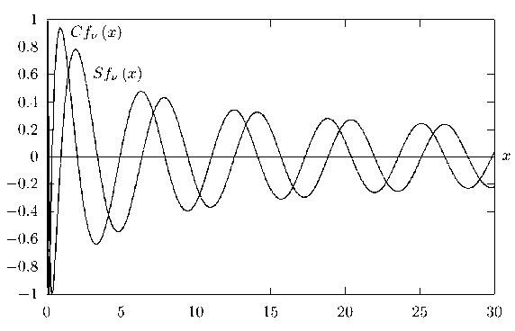
Fig. 3. Functions Sf ^2 ( x ) and Cf 3^2 ( x ) for 0 <  x <  30

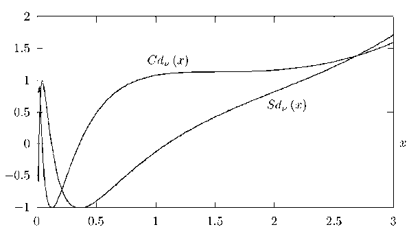
Fig. 4. Functions Sd ^2 ( x ) and Cd ^2 ( x ) for 0 <  x <  3

function. In the above applied cases, the value of the arguments of the Bessel functions lies in the vicinity of unity. The algorithm for their computations is shown to be rapidly converging and gives a very favorable accuracy for as few as eight iterations. Further studies of the asymptotic behavior of these functions are still warranted as they play a great role in boundary valued problems, and integral and differential problems of wave scattering.