On the methodology of checking integral estimates of socio-economic objects

Prediction of the economic growth, development, and social consequences is an important task for government agencies. Using this tool, they can anticipate the consequences of planned actions and correctly adjust their activities with policies to avoid serious socio-economic shocks or accelerate the onset of any positive events.

To assess a territory’s economic and social wellbeing, the GDP indicator has been used for many years (the equivalent for lower-level economic entities is the GRP value) [1; 2]. It is intended to characterize the economic growth dynamics. When assessing business entities, the most developed territories are determined by this metric.

In accordance, the search for “levers” of regulation is an important scientific problem. In other words, the scientific community needs to identify the factors by changing which it is possible to increase or decrease the value of GDP (GRP), and therefore influence economic growth or development.

Such key factors include scientific and technological (in older sources, “scientific and technical”) progress and associated innovative activities of enterprises and organizations [3; 4; 5]. According to several authors [6–11], science and technology are the engine of socio-economic development. Therefore, the state should implement a policy of supporting science and the research sector to increase its competitiveness in the international arena, as well as to improve citizens’ living conditions in a particular territory [12; 13; 14].

In this regard, various economic and mathematical models are being developed [15; 16] (R.M. Solow [8], S. Rebelo [9], K. Arrow [17], P.M. Romer [18], R. Lucas [19], D. Grossman and

E. Helpman [20], K. Freeman and B.-A. Lund-vall [21], C. Griliches [22]). Depending on the indicators chosen and justified by scientists and researchers, they describe functional relationships between economic growth and any economic object (costs for science; amount of research and development works carried out; human capital; enterprises that carry out and implement innovative activities; educational institutions; dynamics of innovative ideas). These models have both a theoretical theoretical justification and some empirical implementation that, to a certain extent, is their approbation and confirmation of the formulated ideas.

Scientists also attempt to conduct a comprehensive assessment of scientific and technological changes in the economic environment. For this purpose, various kinds of “integral” estimates are developed and calculated. An example is the index of the scientific and technical potential of a region, the calculation method of which is published in the works of K.A. Zadumkin and I.A. Kondakov [23], or the assessment of the scientific and technological potential of the territories, presented in an article by a team of authors led by K.A. Gulin [24]. A prominent and fundamental work is the draft “Russian Regional Innovation Ranking”, developed and published from 2012 to 2019 by a team of authors of the Institute for Statistical Studies and Economics of Knowledge, part of the HSE1. This methodology includes an assessment of 37 indicators and has a significant calculation period (7 years).

The mentioned works attempted to assess the cumulative impact of scientific, technological, and innovative development factors on the territories’ socio-economic level (Russia as a separate state, and districts or regions that are part of it, representing similar units of smaller size). As a result of the complexity of the estimates obtained, their interpretation is a kind of conditional unit that characterizes a generalized process or phenomenon (in our case, scientific and technological potential, innovative development, etc.), but does not have an explicit quantitative interpretation that can be obtained during measurement procedures. As a result, the question about the adequacy and reliability of the processes, described by such integral assessments, arises. Their reliability can be confirmed only sometime later, which significantly reduces the significance and practical applicability of such models.

A person often encounters the need to evaluate objects that are characterized by heterogeneous parameters. Most often, such an assessment is carried out intuitively and, as a result, there is a negative result. The use of integral estimates is also associated with several problems, which can be characterized as follows2 [25; 26; 27]:

– need to consider the weight and significance of each of the parameters included in the overall assessment;

– need to specify a way of translating qualitative assessments into quantitative ones;

– distribution of the assessed objects into the corresponding groups, characterized by the magnitude of the levels identified in the study;

– possibility of comparing estimates with the ones that will be obtained in the future (socioeconomic indicators are often non-permanent and may become irrelevant over time, unlike physical quantities that are measured by objects of the natural sciences).

The problematic aspects of integral assessments described above are also indicated in several domestic scientific papers, which attempt to systematize advantages and disadvantages of such approach regarding the interpretation of socio- economic objects. Thus, in the E.N. Volkova’s article, a methodology for characterizing the socioeconomic development of the region is formed and described on the basis of an integral assessment [28]. In the work of E.V. Klyushnikova and E.M. Shitova, the features of constructing integral estimates in accordance with the main stages of modeling are outlined: normalization, aggregation, weighing [29]. Similar studies are being conducted abroad. One of these works is the publication of a team of scientists led by M.-S. Saib [30], in which the authors use an integral indicator to assess the inequality of the population of territories in terms of conditions and factors affecting health.

Among the modern works, special attention should be paid to the publication of A.A. Sidorov [31]. He meticulously systematizes and describes the mathematical nature of the integral approach, thus continuing the work of the famous Russian econometrician S.A. Ayvazyan [32; 33; 34]. In the foreign environment, there are also studies related to the mathematical construction of an integral indicator. Thus, a team of authors led by P. Zhou [35] proposes a variant of aggregating an integral estimate based on the product of adjusted partial values of the included indicators.

Despite the wide variety of works on the use of the integral approach in relation to socio-economic objects, one point is omitted in them – do integral indicators correctly characterize what they are intended to describe? Although nearly all the studies reviewed stipulate that such assessments carry a fair share of indefinite subjectivism.

In this regard, we aim to determine the reliability of artificially derived integral complex estimates by means of mathematical and statistical methods, which, in turn, describe various socioeconomic processes and phenomena.

“Reliability” of the estimates, indicated in the work, means their ability to explicitly describe the processes and phenomena that they should characterize.

To achieve this goal, we have solved several tasks in this work:

– defined and described the methods of mathematical statistics, with the help of which the search for the relationship between economic growth and the assessment of scientific and technological development is carried out;

– formed a sample of data for the calculations indicated in the work;

– carried out and described the results of calculations, based on which the relevant conclusions and recommendations were formulated.

Research methods

One-way analysis of variance

In mathematical statistics, analysis of variance is used to investigate the presence of the influence of qualitative factors on the values of a quantitative indicator. In our case, the resulting indicator will be y : GR P, and for the factor х: хЕ (/ 1Ц / 2 ), (ЛЦ/ 2 ) з S 1 &S 2 &S 3 &S 4 , where 1 1 is the Russian Regional Innovation Index, I ₂ is comprehensive assessment of scientific and technological potential, and (S_n} £ ₌₁ is their constituent sub-indexes.

Using the one-way analysis of variance, we attempt to define whether the difference y in the Russian Federation subjects, observed on k = 4 levels (socio-economic conditions, scientific and technical potential, innovation activity, quality of innovation policy in one case and research and development, personnel, technology, and innovation in the other) is statistically significant.

Algorithm of sample formation for the one-way analysis of variance

The algorithm for selecting elements of four different samples in accordance with levels I1 will be formed based on the ratings of the subjects of the Russian Federation according to the sub-indexes of the Russian Regional Innovation Index. The distributions obtained by scientists and researchers of the ISSEK include four groups that can be characterized as follows (the groups are modeled by the authors of the questioned study, but there is no explicit justification for the boundary values in them; a variant of a possible interpretation is presented below):

I group – cities of federal significance (Moscow, St. Petersburg) that have the best indicators for most statistical metrics characterizing socio-economic development. By their nature, their estimates are several times different from other similar objects (regional territorial units), which is why they are clearly out of the overall distribution picture and look like outliers. In this regard, while conducting the one-way analysis of variance, they will be excluded from our study, which will allow evaluating truly equivalent objects among themselves;

II group – regional territorial entities that have the best values for the assessed characteristics (except for objects included in group I), often exceeding the average national estimates. Such subjects can be regarded the ones that have the studied feature;

III group – the RF regions, which often have values according to S _n estimates that are smaller than the average Russian characteristics; these territories only approach the qualitative level of the studied features I, and therefore they cannot be considered the ones possessing the studied characteristics. It means they should be excluded from further calculations;

IV group – territorial units with the lowest values according to the considered characteristics; they can be characterized by a strong spread of estimates in the context of dynamics, instability of growth rates, and the absence of pronounced trends; in this regard, such objects will not be included in the studied sample.

The algorithm for selecting elements of four different samples in accordance with levels I2 will be formed based on the ratings of the subjects of the Russian Federation by sub-indexes of the assessment of the territories’ scientific and technological potential. The distributions, obtained by scientists and researchers of the VolRC RAS, include five groups (levels: high, above average, average, below average, low), which can be characterized as equally distributed and scaled to a whole dozen (/2 е [0; 10]).

In accordance with the above-mentioned rule of inclusion of observations in the analysis of variance (by analogy with the rating of the subjects of the Russian Federation), we are interested in the “average” and “above average” level groups. In them, as in the previous version, we imply the presence of the considered integrated assessment, therefore, the observation data should be reflected in the change in the dynamics of GRP. The territories included in the high-level sample are unique single objects, and they represent outliers of some kind. The “below average” and “low” level groups include the bulk of observations and, in fact, are identical objects without any prominent features (in 2015, their shares in the sample groups were 93.75; 95; 95, and 98.75%, respectively, in accordance with the selected subindex).

This is the end of the sampling algorithm, and then the algorithm of the one-way analysis of variance continues.

After sampling the regions of the Russian Federation, we determine the number of objects, included in each of the k levels ( k = 4) as the sum of the elements included in the considered set, and denote it by m_n , where n is the ordinal number of the level.

Then we determine the total number ( m ) of objects included in all the samples ( formula 1 ):

т

- I

к т_п

Next, we calculate the average GRP value for each of the formed k groups ( formula 2 ):

У п =

1 ^-1rn_n т_п^ 1 _=г ^{У т}

where y_ni is the GRP value, corresponding to i -region in the sample n .

Next, we will find the average value of the resulting variable y for all available values included in all samples n ( formula 3 ):

1 ч i к ч  1 тт1_п          1 ч 1 к

^ = -1       "-  ' '

The next stage is the search for the sum of squared deviations of the resulting estimates ( y_ni ) by samples from the common average ( у ) ( formula 4 ):

Z k y¹™”

.._.■-■■•■■            (4)

Then, sum of squared deviations of averages by groups ( y^ ) from the total average ( у ) (formula 5 ):

Z k

⁽У П ^- ЙЧ .

n=1

Next, we calculate the residual sum of the squares of the deviations as the sum of the squares of the difference of the resulting values ( y_ni ) from the average values ( у ), included in the same sample ( formula 6 ):

Z k ч i ш_п

/    (У п — УЭ 2 .      (6)

n=1^—'i=1

To check S ² (formula 4), the following equality can be used ( formula 7 ):

^2     ² — C²

^O F + ° res    ° .

Let us calculate the factor variance ( formula 8 ):

2    5F

° ^F = k-1 .

Calculate the residual variance ( formula 9 ):

5 2

2         res

^ res = ~ Г .

m — к

Next, we find the value F_f according to the formula of private factor variance (n²) to residual (a 2es ) (formula 10 ):

°F

Ff = -4" .                  (10)

² . ° res

Using the Fisher–Snedecor distribution, a given level of significance (α), and two degrees of freedom (formula 11 and 12), we can define the metric value F : k df! = k- 1 ;              (11)

df2 = m-k .             (12)

To find F_k , classical Fisher–Snedecor distribution tables, which appear in reference books on mathematical statistics, can be used, but a scientist may encounter a several problems using them. These include the absence of necessary numerical values, which the study is based on. A similar situation associated with the choice of the level of reliability (in the reference literature, there are often only a: a = 0.1||0.05||0.01 ) . Such problem is currently easy to solve using the capabilities of computational computer programs (for example, function “ F_k ” Python “Scipy” libraries).

As a result, it is necessary to compare the values obtained F ^ &F_k (formula 13 ):

F _f >  F _k ^A ,             (13)

where А is the statement that the investigated qualitative features really have an impact on the value of the resulting indicator.

cov

^AJ ^ ху =         ,

СТд-СТу wherecovxy = M ^(хп - ^(ХпЖУп - ^(Уп))) ~ ^ M(xnyn) - in(ynMxn);

M() is the unbiased estimation of the mathematical expectation of the sample;

/() is the average value of the studied observations.

The multiple linear regression model is a tool used in multivariate statistical analysis to describe the relationship of signs (causes) with any result or consequence. Its general form is represented by the analytical formula ( formula 15 ):

У = £o + Pi^i + £2^2 +-----+ £n^n +— ,   (15)

where {^£_n} n=1 is regression coefficients showing the degree of influence of the factor on the resulting feature;

£ 0 is a free parameter of the model that allows the curve to be optimally positioned in space in such a way that the sum of squared deviations (OLS) is the smallest.

To calculate coefficients β , it is convenient to

After building the model itself, it is necessary to evaluate its accuracy and significance. The accuracy of the multiple linear regression model is determined using the coefficient of determination ( R ²), which can be found by the following formula ( formula 17 ):

, SSf

R = s$, where SSf = У  (У; - у)2

^ j=i is the ex-

plained sum of regression squares;

SS = £*_ ^-у?

regression squares;

is the total sum of

j is the ordinal number of the observation included in the generated model.

The closer this metric to one, the better the constructed model approximates the available empirical data.

To compare the accuracy of identical models that differ in the number of regressors, a different metric is used. It is because the coefficient of determination calculated by the method according to formula 17 will always be better with a larger number of parameters. To compare the quality of such regressions, we should use the adjusted R ² ( formula 18 ):

,2 a (1 -R^) • (z- 1) aaj 1 z-n-1

At the final stage, the significance of the constructed model is evaluated. It is determined using Fisher’s F -test. To do this, the required level of significance ( α ) is needed, and we calculate the following characteristics ( formula 19 ):

use the matrix search method ( formula 16 ):

® ■ (

1	XH	^ 12
1	^ 21	X22
1	•^zl	xz2

% 1_П\ ^ 271

X _zn/

/ P₀\ &  ^£ 2

^

W

■^0 = yZ (yt-yt)2 z—1 j=1

^SS-SS_f - is the

residual sum of regression squares;

a number of degrees of freedom;

^ В ■ (X^TX)^-1X^TY

/ SSf SS₀ \ _x I MSf = —f &  MS o = -77^)^ (F_k). \ d/lp df2pj

MS f

^{1 р} MS ₀ .

Determination of ( F _K ) _p happens similarly to the procedure of searching for ( F _K ), however, in this case, instead of dfl (formula 11) and df2 (formula 12), we take accordingly df1_p&df2_p (formula 19). Then, similarly to formula 13, the new corresponding values obtained are compared.

Algorithm for determining the significance of multiple linear regression coefficients

In order to determine the significance of the coefficients of multiple linear regression, the Student’s t -test is used. It allows answering the question: “Can the coefficients obtained in the model be interpreted?”.

The observed values, obtained from the constructed statistical model, are calculated using the standard error of the parameters ( l p ₀ & l p ) £ 0 & £_n accordingly ( formula 20 ):

po o .        pn .. ,,

^=v t=tp°||t/?n.(20)

Standard errors can be found from formula 16 using the matrix A ( formula 21 ):

A = (ХтХуг .(21)

This matrix is square and is determined by the size (k + 1) x (k + 1) . Therefore, its diagonal element can be denoted as a_nn ( formula 22 ):

l p _o ² = MS_oa₀₀ ,

2                   ____ (22)

l p_n = MS_oa_nn, n = 1, к, к = 4 .

The values obtained in formula 21 are compared with the two-way critical point of the Student’s distribution — t k (a; z — n — 1). With |t| >  t k , the corresponding parameter of multiple linear regression is considered statistically significant, the null hypothesis of the form H₀: /?₀11Д п = 0 is rejected.

Algorithm for constructing logistic regression

Using this method, the potential probability of the occurrence of an event can be determined. In our case, the probability of an increase in the GRP dynamics depending on the cumulative annual change of k-factors

In general, the model looks like this ( formula 23 ):

P = P o + p i • Lx i +

+ P 2 ^A% 2 + - + p_n^x_n + - ’

where P is preliminary assessment of the probability of occurrence of a certain event;

{P n ) n=0 is regression coefficients similar to those that characterize the model (formula 15);

{ △ x_n} ^=1 is the values of the annual change of the corresponding factor.

The final transformation (P') can be performed using the sigmoid function, and it looks like this ( formula 24 ):

P' = sigmoid^P^ = ^—-—--^

Algorithm for converting annual GRP dynamics into Boolean function values

If y is a current GRP value, and y ^–1 is a previous one, then ∆ y is favorable dynamics of y by absolute deviation from y ^–1. Then P can be obtained ( formula 25 ):

n Г 1,if Ду >0

Ду ^ -P = [o,if Ду <  0 .        ⁽²⁵⁾

In accordance with the discussed methods, necessary statistical forms are presented below. They were developed by the authors to conduct appropriate statistical assessments, as well as the calculated results and the resulting comments and conclusions.

Table 1. Part of posteriori data set for the one-way analysis of variance

LU (Л z *o X CD 73 c о го > о с го с о СП о СЕ с го ел еЛ 3 СЕ

o' о о. с о го         -~- I   А о го О

со

со

ГО

CD

со см II 6*

СЛ < СЕ О ОС о > о го с о о са го о ел о о о о 73 С го о с о о ел *О с о Е ел ел CD ел ел <

О С

II S"

S S S 1 г со § Ё Ё < ф С О) VD   О О СМ т— Ё Ё О ■5 « CD О S Го CM g 2 $ § "го S ф 1 ^ Ё ° ^ ГО Ё- ^ Е О со о 03 о ГО Ё Ё v) m V) 5^2 ® о о     CZ) 5 з § ° о С Го ^ го § 55 Ё со о го Ё ГО ~ ^ су "о с см — со го го о х ■^   OD ^ X ^ g  i ^ “ с СО "6 го "С —   05 О ° "о -— Ё Е" Ё С° Го Ё о" \ ^ DC S^    ГО i£ч ° В 5 =-■§ 5 8 S £ 5 Е го 2 ш го1 С ф Q ® S   § Ё Ё о ф > -^

^> о ГО     ^ g          II ё   ^ > о с

§

со

LO II е"

ъ  - с       II 5   -S- CD н

со II е"

го о "с о S Го _ 73 ^ ^ С о II si “ с о о <л

со

ГО

ГО

со II е~

О      || О     " О-

со II Е~

ел 73 "> С 13 о О о го ОС ^ Ё S и ° ГО о о о с о с О (Л

CD

ГО

ГО

со см II Е"

с CD Е £2- О CD > о  ■— 73 73       11 С   С го        " -С О го CD ел CD СЕ

II Е"

о 3 73 О О- = 2   5. СП -С о с ел ел О <3

ГО

CD

S

со

го

го

го

со

го

ГО

см со II Е

II Е

3 го о ш го о ел о СЕ

"го го

О

о Ё

о

о

о

о

о го ^

о го ^

О Е го ^

ел с о Е о о о о. Е го ел О о Е 2

ел с о Е о о о £2-Е го ел *О о -Q Е z

Table 2. Results obtained during the analysis of variance

Content of the indicator	Unit of measurement	Symbolic designation	Calculated value
			I 1	I 2
Average GRP value for the group S 1	mil. rub.	У1	1 183 444	1 204 667
Average GRP value for the group S 2	mil. rub.	У2	1 338 762	1 577 121
Average GRP value for the group S 3	mil. rub.	Уз	1 810 813	4 743 038
Average GRP value for the group S 4	mil. rub.	У 4	1 181 169	837 495
Average GRP value for all sample objects	mil. rub.	У	1 327 875	2 237 876
Value of Fisher’s calculated statistics	cond. un.	F f	0.4422	0.4837
Value of Fisher’s critical statistics	cond. un.	F К	2.7218*	4.3468*

* With α = 0.05.

Complied according to Table 1.

To carry out the analysis of variance according to the algorithm described in the first paragraph of the “Research methods”, an array of data was formed ( Tab. 1 ). It presents the values of key subindexes (socio-economic conditions, scientific and technical potential, innovation activity, quality of innovation policy) included in the overall assessment of the “Russian Regional Innovation Ranking”, developed by the ISSEK, and similar indicators (research and development, personnel, technology, innovation) to assess the scientific and technological potential of VolRC RAS. Data are taken in accordance with the latest current calculations carried out at the time of the study described in the 2015 work.

Each of the four groups included those GRP values of the regions. For them, the condition of getting the corresponding index in the significance group was met – group II for the HSE methodology and groups of the “average” and “above average” level for the methodology of VolRC RAS.

In accordance with formulas 1–13 and a posteriori data set, statistical metrics were obtained from table 1 ( Tab. 2 ). They can be used to interpret the analysis of variance carried out in the work to determine the significant impact of the sub-indexes of the studied methods on the level of territories’ economic growth, expressed in the values of the GRP indicator.

During the variance analysis, we tested the hypothesis about the impact and influence of artificially derived integral assessments of the rating of the Russian Regional Innovation Index and estimates of scientific and technological potential on the value of the territories’ gross regional product (dynamics of economic growth). While selecting territories where the corresponding ratings were recorded for four sub-indexes for each method, eight samples were formed respectively, which are characterized by a high manifestation of the processes inherent in one of the four key groups of the studied ratings.

The calculated value of the F-statistics in both cases ( F_{f 1} = 0.4422, F_{f 2} = 0.4837) turned out to be significantly less than the critical value ( F _K1 = 2.7118, F _K2 = 4.3468) with a given reliability level of 5% and the corresponding degrees of freedom obtained (#1_1Н2 = 3 &  №1 = 78 || df2₂ = 7)) (Tab. 2). We may conclude that the differences between the groups of regions, included in the samples by large values (not the maximum possible ones) of the key indicators of the studied methods, are statistically insignificant in relation to the GRP differences. This may indicate two things: either these indicators do not have a significant impact on the regions’ economic growth changes, or the compared comprehensive estimates are mutually dependent.

Table 3. Part of posteriori data set for conducting correlation analysis, building a model of multiple linear and logistic regression

■“

...

...

...

г'

го   О   ^ "о    <С <л    ц5    о r-L со1 2 га    о    S 5   Ё S    c\j cd     с: & ^ ш    о5    СУ 1  1 2 1  1 5 2  о  S го   g ®     5 су             об га     |     го го го        | Ё  §  Ё о     <у)     о ел о   | о. Ё   о о го Ё Ъ    CD О)    "^    О Яго    03    го ОС    .Я    OD Ю . .    м-        С^ О        S ^"" Ё    Е       CD 1    ^    СО       С^ го °   Ё g 55 Ё 2    m    _Я "-Е     ^- го ’ey 8 го га -га -— В го го ?1 1йй£й

"го <

со

со

S

а>

СО

Го

Го

Го

2

Е ° _ ° го II го .£ го

со

m

CD

со

СО

Го

Го

а>

го

Е ° _ g    и го .Е S

со

а

СО

CD

го

CD

Го

Го

CD

Го

Е й

СО

^

^

^

^

\

^

^

7

^

\

& Ё о —-

^

го

2

Го

CD

2

СО

от

Ё ОС О

со

m

со

СО

со

2

Го

2

см

со

со

со

Го

Si

со

со

Го

"го "го

О Е

о

о

о "го СО

О го со

о Ё

о

о

о

Data panel for performing correlation analysis, building multiple linear regression and a logit model

To carry out the selected analyses and modeling options, a statistical panel was formed. It compares the values of changes in the dynamics of the subindexes of the Russian Regional Innovation Ranking and the assessment of the RF territories’ scientific and technological potential ( ∆ n – column 8, etc., Tab. 3 ) with the fact of the GRP dynamics’ growth (column 5, Tab. 3). The generated data were used in the correlation analysis, where information on 2015 sub-indexes was used (column 7, etc., Tab. 3) and the corresponding data characterizing this year’s GRP values (column 4, Tab. 3). The same data set was used in the construction of the multiple linear regression model. To create a logit model, it was necessary to establish the fact of the GRP growth (column 5, Tab. 3) being a positive deviation from the previous year with an absolute deviation of the factors (column 8, etc., Tab. 3), potentially influencing this process.

Correlation analysis

The matrix from Table 4 characterizes the linear relationship between the resulting indicator of the region’s economic growth (GRP) and indicators that are the key sub-indexes of the Russian Regional Innovation Ranking. The data analysis was carried out based on statistics for 2015.

In accordance with the key indicators of the Russian Regional Innovation Ranking and the GRP value, inherent in the studied territories, we have made several relevant conclusions.

Gross regional product

There is a linear relationship between socioeconomic conditions of work. A response from the values of the indicator characterizing the scientific and technical potential was revealed. Indicators describing the level of innovation activity and the quality of innovation policy have almost no linear effect on the growth or decline of economic growth in the regions of the Russian Federation.

Socio-economic conditions of innovation activity

This indicator strongly correlates with the values of the indicator characterizing the scientific and technical potential of the RF regions. This may be caused by high correlation between GRP and scientific and technical potential. There is a connection with the indicators of innovation activity, but it is insignificant with the quality of innovation policy.

Scientific and technical potential

The values of this indicator correlate with the values of indicators characterizing the innovative activity of the Russian regions. There is a stronger relationship with the quality of innovation policy than in previous indicators.

Scientific and technological potential

These indicators are more correlated with each other than the rest.

General conclusion

There is a pronounced interdependence between the studied metrics. It confirms the conclusions obtained during the analysis of variance, which showed the absence of a statistically significant

Table 4. The results of the correlation analysis carried out using the ISSEK methodology

	GRP	n 1	n 2	n 3	n 4
GRP	1	0.6669	0.4540	0.2652	0.1571
n 1	0.6669	1	0.5905	0.3935	0.2289
n 2	0.4540	0.5905	1	0.4007	0.2897
n 3	0.2652	0.3935	0.4007	1	0.4892
n 4	0.1571	0.2289	0.2897	0.4892	1
Complied according to Table 3.

Table 5. Results of the correlation analysis held according to the VolRC RAS methodology

GRP n1 n2 n3 n4 GRP 1 0.6674 0.6862 0.4558 0.3051 n1 0.6674 1 0.8034 0.8205 0.3481 n2 0.6862 0.8034 1 0.6430 0.2631 n3 0.4558 0.8205 0.6430 1 0.3783 n4 0.3051 0.3481 0.2631 0.3783 1 Complied according to Table 3. difference between the GRP value of objects belonging to different categorical groups according to the levels of regions’ innovative development.

The matrix from Table 5 characterizes the linear relationship between GRP and the key sub-indexes of the rating, which assesses the territories’ scientific and technological potential (2015).

• 1)    Gross regional product

In accordance with the practice of econometric modeling, the relationship of GRP with indicators, which are chosen as predictors, is weak and cannot be properly used to predict or interpret the movement of the dynamics of the resulting estimate as a linear response from them.

• 2)    Research and developments

The group of indicators that has the highest correlating values for all the studied sets of subindexes of the VolRC RAS methodology. Its significant level is observed for the indicators of the “Technology” (0.8) and “Innovation” (0.82) groups. At the same time, these groups correlate with each other much less (0.64). Perhaps, it can be successfully used to build a model of multiple linear regression, where “Research and development” will act as the resulting estimate.

• 3)    Technologies

Weak linear relationship with the group of indicators “Innovation” and “Personnel”.

• 4)    Innovation

There is practically no linear relationship with the last group of indicators characterizing the abstract systematization of scientific personnel.

General conclusion

There is a situation similar to the case with the correlation analysis conducted according to the rating of the assessment of innovation development of the RF subjects. Specifically, it is necessary to highlight the relationship of the indicators in the “Technology” and “Innovation” groups with “Research and development”. Nevertheless, there is still a strong interdependence of some metrics with others used to calculate the final resulting estimate, It indicates the need to use an effective method of searching for weights when forming the final calculation, or reducing the dimension of a number of predictors by eliminating irrelevant factors.

Multiple linear regression

Table 6 shows the main statistical metrics of the results obtained according to the statistical models of multiple linear regression constructed in the work. Namely, parameters of the regression model, both basic and modified; coefficients of determination and their adjusted estimate; calculated and critical Fisher F -statistics at a given reliability level of 5% and assessment of the significance of the obtained model parameters using t -statistics.

The graph of actual 2015 values of the regions’ GRP, sorted by ascending values of the sub-index of the Rating of Innovation Development of the Russian subjects ( Fig. 1 ) that characterize the socio-economic conditions for the implementation and carrying out of innovative activities in the country’s territorial subjects, is given below. This

Figure 1. Graphical visualization of regression modeling using the HSE methodology

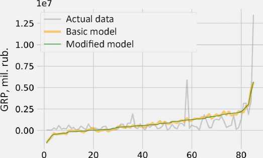
Observations (sorted by the indicator “Soc.-ec. cond. of inn. act., 2015”)

Complied according to Table 3.

ranking is caused by the presence of the GRP values approximated by the only parameter, specified before, in the model. In this regard, we can try to graphically display the dependence of the studied value (gross regional product) on a specifically established predictor (integral assessment of socioeconomic conditions of innovation activity).

Since the value F of the calculated statistics ((F f )_p = 16.3967) exceeds the critical value ((^ k ) p = 2.4859) at the given significance level of 5%, then the hypothesis that all predictors in the regression model are simultaneously equal to zero is rejected, i.e. the constructed basic statistical model is statistically significant ( Tab. 6 ). However, with a more detailed examination of it and tests for the obtained parameters, biased estimates were identified into t -statistics. Among five coefficients, including “intercept”, only two were significant: “intercept” and the parameter β ₁ , which characterizes the socio-economic conditions of innovation activity. Insignificant parameters ( β ₂ – scientific and technical potential; β ₃ – innovation activity;

β ₄ – quality of innovation policy) were excluded from the modified model, and a new statistical model, corresponding to the conditions of F and t statistics was obtained. It was also possible to increase the value of the adjusted R ² from 0.42 to 0.44.

Similarly to the previous one, the results of modeling according to the methodology of VolRC RAS ( Fig. 2 ) are presented. The sorting of the resulting and actual GRP values was carried out according to the “Frames” indicator in accordance with the highest value obtained when calculating its t -statistics (3.1554).

During the initial examination, we may note that the regressions constructed according to the second studied indicator ( I ₂ ) more accurately repeat the dynamics of actual GRP values. This is also evidenced by the adjusted coefficient of determination R a _d j' (I 2 ) = 0.4962 larger R^j (Ю = 0.4380 . It may be caused by the decrease in the dimension of the indicators included in the second methodology. That is why the averaging of the studied estimates is not so pronounced. To some extent, this is

Table 6. Regression modeling results

Indicator’s name	Symbolic designation	Calculated value
		/ i	/ 2
1. Basic regression model: у = p0 + pixi + p 2 x 2 + P 3 x 3 + P ^ x ^
ул = -3964780.87 + 11310999.28x 1 + 1854358.59x 2 - 173667.55x 3 - 50769.69x 4
у, = -663095.39 + 564364.88x 1 + 533221.86x 2 - 335361.73x 3 + 201959.81x 4
intercept	ft o	-3 964 780.9	-663 095.39
Calculated t -statistics for ft 0	4	6.2250	2.7310
Socio-economic conditions of innovation activity / Research and development	ft l	11 310 999	564 364.88
Calculated t -statistics for ft		5.8615	3.0278
Scientific and technical potential / Personnel	ft 2	1 854 358.6	533 221.86
Calculated t -statistics for ft	^2	0.9157	3.1671
Innovation activities / Technologies	ft 3	-173 667.55	-335 361.73
Calculated t -statistics for ft3	^3	0.1326	2.1266
Quality of innovation policy / Innovations	ft 4	-50 769.69	201 959.81
Calculated t -statistics for ft4	^4	0.0564	1.4406
Critical point of Student’s distribution	t k	1.9901	1.9921
Coefficient of determination	R 2	0.4505	0.5437
Adjusted coefficient of determination	R 2dj	0.4230	0.5194
Fisher’s F -criterion, calculated	№) p	16.3967	22.3439
Critical value of Fisher’s distribution	(ft) p	2.4859	2.4936
2. Modified regression model: y / i = p0 ' + p1 ' x1
у ' = -3813320.76 + 12243723.31x 1
New intercept	ft o'	-3 813 320.76
Calculated t -statistics for ft0 '		6.5117
Socio-economic conditions of innovation activity (unbiased assessment)	ft l'	12 243 723.31
Calculated t -statistics for ft l	4'	8.1531
New critical point of Student’s distribution	t k'	1.9890
New coefficient of determination	R 2 '	0.4447
New adjusted coefficient of determination	R ^dj'	0.4380
New Fisher’s F -criterion, calculated	(ft)p'	66.4736
New critical value of Fisher’s distribution	(ft)p'	3.9560
3. Modified regression model: y / 2 = p0 ' + p1 ' x1 + P2 ' x2
у / , = -393469.1 + 346573.61x 1 + 543161.88x 2
New intercept	ft o'	-393 469.10
Calculated t -statistics for ft0 '	4'	2.0592
Research and development (unbiased assessment)	ft l'	346 573.61
Calculated t -statistics for ft 1'	4'	2.4416
Personnel (unbiased assessment)	ft 2	543 161.88
Calculated t -statistics for ft2 '	t g , '	3.1554
New critical point of Student’s distribution	t k'	1.9912
New coefficient of determination	R 2 '	0.5090
New adjusted coefficient of determination	R ^dj'	0.4962
New Fisher’s F -criterion, calculated	(ft)p'	39.9059
New critical value ofFisher’s distribution	(ft)p'	3.1154
Complied according to Table 3.

Figure 2. Graphical visualization of regression modeling by the VolRC RAS methodology

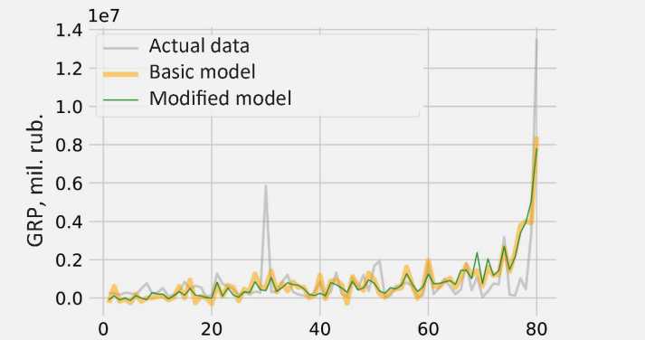
Observations (sorted by the indicator “Frames, 2015”)

Complied according to Table 3.

an advantage of the VolRC RAS methodology in relation to the one developed by HSE researchers.

By modified regression y ‘ 2 in comparison with y ‘ 1 , we should note that it has a greater number of degrees of freedom (per predictor). It provides appropriate flexibility and independence in predicting the resulting estimate.

Conducted research once again showed the absence of a significant influence of factors appearing in the Russian Regional Innovation Index and the Index of Scientific and Technological Potential, which, in turn, determine scientific and technological development and innovative activity in Russia. Although, in accordance with the provisions of the economic theory, they should have a direct impact on the dynamics of economic growth and development of the business entity. Considering all this, we may conclude that artificially derived indicators do not adequately characterize the territories’ scientific and technological potential, innovative activities, and innovative policies carried out in a particular region.

Table 7 provides the main estimates based on the developed and tested logit model that predicts the probability of the GRP growth in accordance with the absolute change in the sub-indexes of the rating of the Russian Regional Innovation Index and the assessment of scientific and technological potential. The basic logistic regression includes all four key indicators available in the rating, but due to the model’s inconsistency (insignificance according to Fisher statistics and coefficients for the indicators included in the t -statistics model), there is no modification of it.

According to the obtained values of the F -test (Table 7), the compiled models are statistically insignificant, i.e. the cumulative change in the model parameters characterizing the change of socio-economic conditions of innovation activity, scientific and technical potential, innovation activity, quality of innovation policy or innovations, technology, personnel and research, and development in the regions does not manifest itself in a change in the GRP dynamics.

Table 7. Results of regression modeling of the logit model

Indicator’s name	Symbolic designation	Calculated value
		/ 1	/ 2
Logistic regression model: p' - ^—(^^^^з^)
P',                                       1
* 1    1 + g -(0.7466-1.425244 1 + 1.8070-Дх 2 -1.7907-Дх 3 +0.3162-Дх 4 )
1 P ', = -----:----------------—--------:--------—
* 2     1 + g -(0.7111+0.077S4x 1 + 0.14S24x 2 -0.13214x 3 +0.13734x 4 )
intercept	P 0	0.7466	-0.7111
Calculated t -statistics for p0	^ Pd	13.4386	11.3365
Changes of socio-economic conditions of innovation activity	P 1	-1.4252	0.0775
Calculated t -statistics for P 1	t p i	1.0734	0.3926
Changes of scientific and technical potential	P 2	1.8070	0.1452
Calculated t -statistics for p2	t p 2	1.2301	0.4324
Changes of innovation activity	P 3	-1.7907	-0.1321
Calculated t -statistics for p3	^3	1.8590	2.0185
Changes of the quality of innovation policy	P 4	0.3162	0.1373
Calculated t -statistics for p4	^4	0.4394	1.9119
Critical point of Student’s distribution	^ k	1.9908	1.9921
Fisher’s F -criterion, calculated	CF f ) p	1.9378	1.4182
Critical value of Fisher’s distribution	Фк)р	2.4889	2.4937
Complied according to Table 3.

Figure 3. Assessment of the reliability of integrated assessments of socio-economic objects

1. Linking the integrated assessment to the resulting indicator, which will be influenced by changing integral assessment
2.1. One-way analysis of variance	2.2. Correlation analysis	2.3. Multiple linear regression	2.4. Logistic regression of changes in dynamics	2.5. Other methods of statistical analysis and data processing

Source: own compilation.

an answer. As a result, we cannot take appropriate measures to eliminate negative effects.

We should also mention the specifics of socioeconomic indicators. Unlike the natural sciences, simulations based on such estimates cannot be reproduced for testing in laboratory conditions. In this regard, the reliability and adequacy of such models is based only on theoretical propositions that may turn out to be both correct and refuted over time.

In addition, let us note that the nature of socioeconomic metrics is unstable and changeable. That is, the same indicator can mean different things at different times. These indicators are narrow-profile, and they characterize various unique objects, which cannot be stated about the mass of a material object, the speed of movement, the presence of a certain set of genes and other things, inherent in the objects of natural sciences research.

Largely, the bias of the estimates obtained is caused by the fact that duplicate (highly correlated) indicators are used in their compilation. With their significant share in the final calculation, the value of the integral indicator is averaged, and it does not reflect the differentiation in the totality of the studied objects.

To avoid such problems, discussed statistical methods can be used. At the same time, they can be

applied separately and in combination, complementing and confirming the corresponding statistical hypotheses, or indicating the need for additional research ( Fig. 3 ).

In accordance with figure 3, a stable indicator should be determined first. It is recorded in statistical reports without any changes and will potentially be used. Then we need to establish a connection between it and the integral assessment (as shown in the work, it can be done by means of variance, correlation, and regression analysis), which will allow assessing the reliability of the developed integral methodology. The more statistical tests are applied to the assessment of the relationship between the resulting metric and the integral one, and the more coincidences there are between them, the more stable and reliable the conclusions are, which can be obtained when comparing socio-economic objects evaluated using integral methods, are.

Methods designed to reduce the dimensionality and the number of studied processes and phenomena are also important in solving this problem. The final model should include significant factors, which is shown by the methods discussed.

We should also mention the approach associated with the use of narrow-profile econometric models that consider spatial locations of the studied object;

time lag of the manifestation of an event; the nonlinear nature of the process, etc. These problems and questions are not trivial, and they are more applicable to metrics and indicators that can be removed from the studied object. In case of assessments similar to integral or comprehensive one, such approach is unlikely to be successful, since it includes things that occur independently

in various manifestations. It will just confuse the researcher during mathematical modeling.

The materials of the publication might be used by experts specializing in scientific and technological development, innovation, and technological promotion, as well as by scientists and researchers engaged in statistical processing and data analysis.