On the Signal-Image Intensity-Curvature Content

Within the context of optimization of interpolation procedures, the literature is rich of measures of the signal-image energy (i.e. [1-3]). The literature is missing though of an approach which quantifies the content of the signal-image through the combined information content of the values of both of the signal intensity and the total curvature of the signal-image. As far as the total curvature is concerned, the literature reports on examples of techniques employed to calculate derivatives of the signal-image on the basis of convolution operators like: the gradient [4], compact finite differences [5] and multidimensional derivative filters [6], and nonetheless to mention, the Sobel operator [7] used to calculate the first order derivative. The biomedical problem being addressed in this manuscript is that one of defining novel measures of the signal-image content which: make use of the total curvature of the signal-image; and at the same time calculate the total curvature using all of the second order derivatives of the Hessian of the model function fitted to the data. The engineering innovation provided through this manuscript is that one of combining the value of the signal with the value of the total curvature. It is therefore possible to establish a measure of the intensity-curvature content level of the signal, which distinguishes concave signals from convex signals, thus obtaining novel local properties of the signal-image which are called intensitycurvature functional and intensity-curvature measure.

Resent research in signal-image interpolation [8, 9] shows the feasibility of the improvement of the approximation characteristics of a set of interpolation functions (under the same methodological approach) through the use of the intensity-curvature functional. This manuscript is intended to provide to the reader with the math details of the intensity-curvature functional and the intensity-curvature measures, as well as with some qualitative results obtained with the formulations herein reported when studying the bivariate linear, the trivariate cubic Lagrange interpolation functions and the monodimensional quadratic and cubic B-Spline and the cubic Lagrange polynomials. In section II of this manuscript the formulae are presented, in section III the results are reported and in section IV the discussion highlights the features of the novel content measure of the signalimage herein described thereby stressing on the significance of the results in biomedical image processing.

• II.    THEORY

Noteworthy the following two premises: (i) one is that the model function needs to have existing and non null second order derivatives, and (ii) the other one is that all of the second order derivatives of the model function are included (with respect to all of the dimensional variables) in the calculation of the total curvature. Given a model function f(x), with x = x1, or x = (x1, x2) or x = (x1, x2, x3) or more generally: x = (x1, x2...xn), fitting the discrete sequel of digital values the signal-image is composed of, the intensity-curvature functional is defined as:

AE( x ) = { S i J f( 0 ) • [ (d² ( f( x ) ) dx dx )| x o } /

{s i J f( 0 ) • [ (d² (f( x )) /dx i dX j )] x = x }                     (1)

The numerator of (1) is called intensity-curvature term before interpolation and the denominator of (1) is called the intensity-curvature term after interpolation. In other words, the term at the numerator calculates both of the value of the model function and all of the derivatives of the Hessian of the model function at the spatial-temporal location x = 0, while the term at the denominator calculates both of the value of the model function and all of the derivatives of the Hessian of the model function at the spatial-temporal location x = x (intra-pixel location). The intensity-curvature term before interpolation [8, 9] is employed to measure the intensity-curvature content level of the non-interpolated signal (given f(x) as model function). The formulations (2) through (4) define the intensity- curvature terms before interpolation in 1D, 2D and 3D:

E o (x) = J [f(0) • (d² ( f(x)) /dx²)] _x=o dx                   (2)

E o (x, y) = J J f(0, 0) • [ (d² ( f(x, y)) /dx²) + (d² ( f(x, y)) /dy²) + (d² ( f(x, y) ) /dxdy) + (d² ( f(x, y) ) /dydx)] (x, y = (0, 0) dx dy                                                     (3)

E o (x, y, z) = J J J f(0, 0, 0) • [ (d² ( f(x, y, z)) /dx²) + (d² ( f(x, y, z)) /dy²) + (d² ( f(x, y, z)) /dz²) + (d² ( f(x, y, z)) /dxdy) + (d² ( f(x, y, z)) /dydx) + (d² ( f(x, y, z)) /dxdz) + (d² ( f(x, y, z) ) /dzdx) + (d² ( f(x, y, z) ) /dydz) + (d^{2 ( f(x}, y, ^z) ) dzdyi^ x,y,z) = (0,0,0) ^dx dy dz                ⁽⁴⁾

The formulations (5) through (7) define the intensitycurvature terms after interpolation in 1D, 2D and 3D:

E in (x) = J [f(x) • (d² ( f(x) ) dv)| x x dx                  (5)

E iN ^(x, y) =^{J J f(x,} y • ^{[ (}d^{2 ( f(x}, y) ) /dx²⁾ + (d^{2 ( f(x}, y) ) /dy²) + (d² ( f(x, y)) /dxdy) + (d² ( f(x, y) ) /dydx)] _(x, _y) = (x, y) dx dy                                                     (6)

E in (x, y, z) = J J J f(x, y, z) • [ (d² ( f(x, y, z)) /dx²) + (d² ( f(x, y, z)) /dy²) + (d² ( f(x, y, z)) /dz²) + (d² ( f(x, y, z)) /dxdy) + (d² ( f(x, y, z)) /dydx) + (d² ( f(x, y, z)) /dxdz) + (d² ( f(x, y, z) ) /dzdx) + (d² ( f(x, y, z) ) /dydz) + (d^{2 (} ^x У^{, z)} ) /dzdy)] (x, y, z) = (x, y, z) dx dy dz                ⁽⁷⁾

From (1) through (7) the following intensity-curvature measures were derived through the works presented in [8] using the Sub-pixel Efficacy Region. As far as regards the one-dimensional quadratic B-Spline and the one-dimensional cubic Lagrange interpolation functions, the intensity-curvature measure is:

EIN(xSRE - x0) / EIN(xSRE)(8)

As far as regards the one-dimensional cubic B-Spline, the intensity-curvature measure is:

AE(xsre - x0) / AE(xsre)(9)

And, as far as regards the bivariate linear interpolation function, the intensity-curvature measure is:

EIN((xSRE, ySRE) - (x0, y0)) / EIN(xSRE, ySRE)(10)

• III.    QUALITATIVE RESULTS

This section reports on the results of the calculation of the intensity-curvature measures shown in (1), (8), (9) and (10), when re-sampling in one, two and three axial dimensions. The quadratic B-Spline, the cubic B-Spline and also the cubic Lagrange polynomials are fitted to 2D images, when re-sampling in one direction. The bivariate linear interpolation function is fitted to a 2D image when re-sampling in two axial directions. Additionally, results were obtained fitting the trivariate cubic Lagrange model function to a 3D image when resampling in three directions. All of the misplacements have been used in order to apply virtual shift-rotations to the images [9].

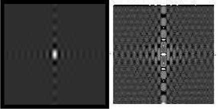
An 139 × 139 pixels image with pixel size 1.0 mm × 1.0 mm is shown in Fig. 1(a), whereas in (b), (c) and (d) of Fig. 1 is shown the intensity-curvature measure (8) obtained with a parametric quadratic B-Spline polynomial (see (b)), the intensity-curvature measure (9) obtained with a cubic B-Spline polynomial (see (c)), and the intensity-curvature measure (8) obtained with a cubic Lagrange polynomial (see (d)). Figs. 1(b), 1(c) and 1(d) are different, showing that the intensity-curvature measure is not the same across the three images. Resampling was of a misplacement of 0.1 mm in all of Figs. 1(b), 1(c) and 1(d).

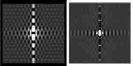
This result is suggestive that the model function fitted to the signal-image is a determinant of the intensitycurvature content which is detectable through the intensity-curvature measure. Fig. 2 shows in (a), (b) and (c) the intensity-curvature measure (8) obtained when fitting to the image seen in Fig. 1(a), the quadratic onedimensional B-Spline (a), the intensity-curvature measures (9) and (8) obtained when fitting the onedimensional cubic B-Spline (b) and the one-dimensional cubic Lagrange (c) respectively, when re-sampling in one axial direction with a misplacement of 0.3 mm.

In one of the two cases shown in Fig. 3, the magnitude of the misplacement does have an effect on the map of the intensity-curvature measures (8) and (9) when re-sampling with the one-dimensional cubic Lagrange and the one-dimensional cubic B-Spline interpolation functions respectively. The intensitycurvature image content is not measured to be the same (see (b) versus (d)). The model function is the onedimensional cubic B-Spline in (b) and the onedimensional cubic Lagrange in (c). Re-sampling is of the misplacement of 0.3 mm in (d) where the model function is the one-dimensional cubic B-Spline, and in (e) where the model function is the one-dimensional cubic Lagrange.

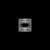
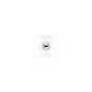
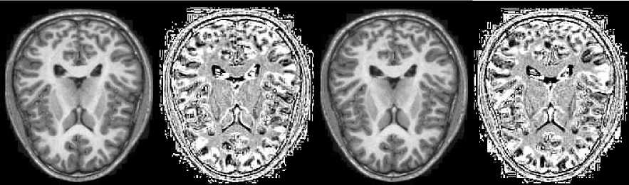
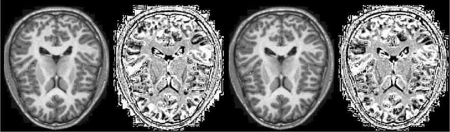
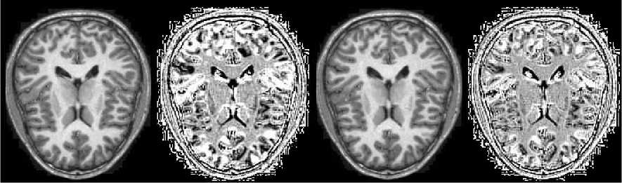
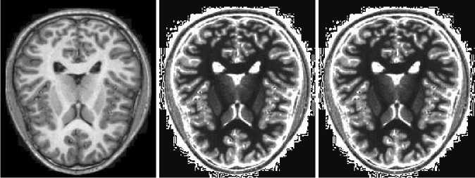
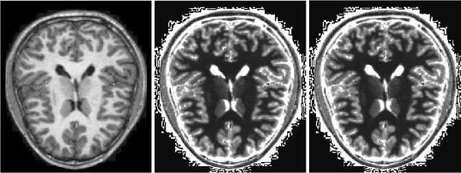
Data seen in Fig. 4 are from the portion of the MRI volume comprising of 6 slices and the intensity- curvature functional was obtained through the use of the trivariate cubic Lagrange function employed to fit the three-dimensional image. The value of the misplacement where the signal is re-sampled is 0.1 mm along all of x, y and z axis. Data seen in Fig. 5 were obtained through the use of the intensity-curvature measure (10) when fitting the bivariate linear interpolation function to the image data. Two MRI images are shown in (a) and (d); and in (b) and (c) are shown the corresponding intensitycurvature measures (10) when re-sampling a misplacement of 0.1 mm and 0.3 mm respectively along both of the x and y axis.

(a)                        (b)

(c)                        (d)

Figure 1. In (a), a two-dimensional image 139 × 139 pixels (1.0 mm × 1.0 mm) padded with 5 pixels along the 4 edges, in (b), in (c) and in (d) the intensity-curvature measures calculated when fitting the onedimensional quadratic B-Spline and using (8) (see (b)), the onedimensional cubic B-Spline and using (9) (see (c)), and the onedimensional cubic Lagrange and using (8) (see (d)), when re-sampling a misplacement of 0.1 mm along the x axis (horizontal). The formulae of the aforementioned polynomials are found in [8].

Similarly in (e) and in (f) are shown the intensitycurvature functional of the image seen in (d) for a misplacement of 0.1 mm (e) and 0.3 mm (f) respectively along both of the x and y axis. In the two cases shown in Fig. 5, the magnitude of the misplacement does not have an effect on the map of the intensity-curvature measure and so the intensity-curvature content is measured to be the same in both of the cases presented (re-sampling of 0.1 mm and 0.3 mm).

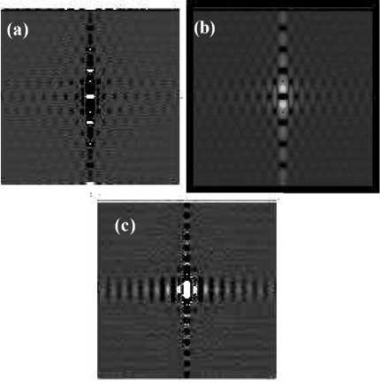
Figure 2. Two-dimensional intensity-curvature measures of the image seen in Fig. 1(a). The intensity-curvature measures are obtained with one-dimensional model functions: quadratic B-Spline and using (8) (shown in (a)), cubic B-Spline and using (9) (shown in (b)), and cubic Lagrange and using (8) (shown in (c)); when re-sampling the image in Fig. 1(a) of a misplacement of 0.3 mm along the x axis.

(a)           (b)         (c)

(d)           (e)

Figure 3. The calculation of the intensity-curvature measure with changing misplacements. In (a) a two-dimensional light source image 65 × 65 pixels (1.0 mm × 1.0 mm), in (b) and (c) the intensitycurvature measure obtained when re-sampling the image in (a) of a misplacement of 0.1 mm along the x axis with the one-dimensional cubic B-Spline and using (9) (see (b)); and the one-dimensional cubic Lagrange and using (8) (see (c)). The intensity-curvature measure calculated with (9) when re-sampling the image in (a) of a misplacement of 0.3 mm is shown in (d) (cubic B-Spline). And in (e) (cubic Lagrange) is shown the intensity-curvature measure obtained using (8).

(a)                         (b)                         (c)                    (d)

(e)                          (f)                           (g)                      (h)

(i)                            (j)                             (k)                        (l)

Figure 4. The Magnetic Resonance Imaging (MRI) three dimensional volume shown in (a), (c), (e), (g), (i), (k) belongs to the OASIS database: org [13-18]. And the corresponding intensity-curvature functional slice by slice are shown in (b), (d), (f), (h), (j), (l). Voxels are 1.0 mm × 1.0 mm × 1.00 mm along the edges: x, y and z respectively. The matrix size on the 2D plane is 176 × 208 pixels. The intensity-curvature functional images were calculated with the trivariate cubic Lagrange formula [9].

Even though the model function introduces bias because of its arbitrary choice; it is true that the same proposed approach is extendible to any model function given the constraint property of second order differentiability of the math model.

Observation of the images in Fig. 1 through Fig. 5 yields the following major results. Figs. 1, 2 and 3 provides with a practical demonstration of the change in intensity-curvature content consistently with the change in the re-sampling location, given that is it observed a change in the values of the intensity-curvature measure for example when looking at the difference between Fig. 3(b) (re-sampling of 0.1 mm) and Fig. 3(d) (re-sampling of 0.3 mm). Similar results are observable when comparing the intensity-curvature measure maps in Figs. 1 and 2. It is worth noting the consistency observable in Fig. 3 in that the intensity-curvature measure is zero when the signal is zero whereas it provides with an evidence of non null values otherwise.

Additionally, in Figs. 1(b), 1(c), and 1(d), 2(a), 2(b) and 2(c), the quadratic and cubic B-Splines as well as the cubic Lagrange polynomials allows the calculation of an intensity-curvature measure map which is well correlated with the image features shown in Fig. 1(a). This is also remarkably seen in Fig. 4 (intensitycurvature functional) and Fig. 5 (intensity-curvature measure). Additionally, in Figs. 1(b), 1(c), and 1(d), 2(a), 2(b) and 2(c), it is observable that the values of the intensity-curvature measure follow the patterns of signal intensity observed in the original image seen in Fig. 1(a). A similar observation can be made for Figs. 5(b), 5(d), 5(e), 5(f) in relationship to the MRI seen in Figs. 5(a) and 5(d).

• IV.    DISCUSSION AND CONCLUSION

Only in recent years adaptive re-sampling has been recognized as the mean to progress in signal-image interpolation to the extent of generating novel approximation paradigms with optimized interpolation error [10-12]. The specific reason why the intensitycurvature functional comprises of the total curvature of the model function descends from the intent of the unifying theory [8].

(b)

(a)

(c)

(d)

(e)

(f)

Figure 5. The images in (a) and (d) are the original MRI with a 176 × 208 pixels' matrix which pixel size is 1.0 mm × 1.0 mm (OASIS database: [13-18]). The images in (b) and (e) are the two intensity-curvature measure (10) obtained when re-sampling the misplacement of 0.1 mm along both of x and y axis, whereas the images in (c) and (f) are the two intensity-curvature measure (10) obtained when re-sampling the misplacement of 0.3 mm along both of x and y axis. The four intensity-curvature measure images were obtained when fitting the bivariate linear interpolation function to the original images shown in (a) and (d).

• A.    The Philosophy of Thought

The philosophy of thought upon which the conception of the intensity-curvature functional descends from, addresses the general problem of discontinuity (digital) versus continuity (mathematics). Given a discrete sequel of samples obtained at a given sampling frequency, the problem consists in that of bringing continuity to the samples which otherwise would remain discontinuous in their nature. Within the aforementioned extent, the use of a model formula like the B-Spline, for instance, to model the signal-image data on a pixel-by-pixel basis, brings continuity to the discrete sequel of samples. Logically, one implication of the continuity in the signal-image is that local properties of the signal-image can be formulated. The locality of the property brings the advantage of its mathematical definition and characterization for each value of the real numbers where the model function is defined. Specifically, the math definition and characterization is possible in the entire interval where the model function is defined. In this paper the intensity-curvature functional and the intensity-curvature measures are the properties which are presented, and such properties embed, under the fulfilled assumption of second order differentiability of the model function, the capability to be local to the model function and thus local to the signal-image (defined for each x belonging to the interval of definition of the model function).

The intensity-curvature functional and the consequential intensity-curvature measures are therefore local properties of the signal-image and as such they are continuous in the interval of definition of the model function fitted to the signal-image. Having clarified the mathematical nature of the philosophy of thought (the descending properties and implications will be addressed in the next section), it is here reinforced what already presented in other venue [9]. Indeed, another very basic property of the signal-image made continuous through fitting a model function, is the total curvature calculated through the sum of all of the second-order derivatives of the Hessian of the model function fitted to the signalimage. However, the discussion of the properties of the total curvature is beyond the scope of the present manuscript.

Before the concluding remarks, it is worth noting that the intensity-curvature functional has been earlier invented [19] when reporting on the approximate nature of the bivariate linear interpolation function. It is also worth recalling that the improvements of the approximation properties of several mathematical functions of diverse degree and dimensionality have been reported and studied extensively in [8] and such improvements were obtained through the use of the intensity-curvature functional.

• B.    Significance of the Intensity-Curvature Functional

On the basis of the total curvature of the model function, the intent is that one of re-mapping the relationship existing between the dependent and the independent variables of the model function. There are two facts of relevance worth mentioning in relationship to the significance of the intensity-curvature functional. One is that novel interpolation paradigms called SRE-based interpolation functions have been devised through the use of the intensity-curvature functional [8]. And the other fact is that through the intensity-curvature functional it is possible to derive additional novel classes of interpolation functions called: (i) resilient-curvature and (ii) classic-resilient-curvature (hybrid) interpolation functions [9]. The aforementioned two facts provide with the significance of the engineering solution herein presented which has implications in the realm of biomedical engineering. The signal-image intensitycurvature content introduced in this paper: the intensitycurvature functional and the intensity-curvature measures, are calculated in the image space on the basis of the ratio between terms which are made of the multiplication of the signal-image times the total curvature. The term at the numerator of the intensitycurvature functional is calculated at the grid point in absence of re-sampling, whereas the term of the intensity-curvature functional at the denominator is calculated at the misplacement where the signal is resampled with the model function chosen in order to fit the data.

On the basis of the images of the intensity-curvature functional and the intensity-curvature measures presented here, two major results can be highlighted. One is that the intensity-curvature functional and the intensity-curvature measures are dependent on the math of the function fitting the data. And the other one is that both of the intensity-curvature functional and the intensity-curvature measures are dependent on the resampling location where they are calculated. To an observer though, the intensity-curvature functional and the intensity-curvature measures demand the unit analysis. The following explanation is in order. Both of intensity-curvature terms before and after interpolation are measurable through the unit made through the multiplication between: (i) the unit associated with the signal-image intensity and (ii) radians (since the total curvature is geometrically the arctangent of the angle formed by the tangent-line to the first order derivative of the model function). Therefore the intensity-curvature functional is a dimensionless quantity (it is a pure number).

• C.    Conclusion

In conclusion it is herein presented a novel method to measure the content of a signal-image through the use of the discrete samples and the total curvature of the math model fitted to the data. The biomedical engineering problem of formulating a novel measure of signal-image content is thus solved through the intensity-curvature functional and the intensity-curvature measures, which make the engineering innovative solution to the problem herein stated.

The significance of the results is to the extent of the application of the intensity-curvature functional and the intensity-curvature measures to the improvement of the approximation properties of the interpolation functions [8, 9].

A cknowledgment

Hereto publishing findings that benefit from OASIS data , we are due to mention the following grant numbers: P50 AG05681, P01 AG03991, R01 AG021910, P20 MH071616, U24 RR021382 . The author is very grateful to Professor Fadi P. Deek, New Jersey Institute of Technology, U.S.A., for the invaluable suggestions provided during the developmental efforts of this research. Formulae (2) through (7) are reprinted with permission from [9].