On the Use of Time–Frequency Reassignment and SVM-Based Classifier for Audio Surveillance Applications

Published Online November 2014 in MECS

Generally, automatic sound recognition (ASR) has been interested on the analysis of speech and music but now some efforts have been emerged on detecting and classifying environmental sounds [1-2-3-4] .This paper is interested in the environmental sounds classification. The purpose is the identification of some current life sounds class. Among the possible applications [5-6-7-8], we quote: the cars classification according to their noise, the fire arms sounds identification to warn the police, the distress sounds identification for the remote monitoring systems and medical security [9]. Many previous works on environmental sounds classification have proposed a variety of acoustic features such as MFCCs, frequency roll-off, spectral centroid, zero-crossing, energy, Linear-Frequencies Cepstral Coefficients (LFCCs), parameters from wavelet transform. These descriptors can be used as a combination of some, or even all, of these 1-D audio features together, but sometimes the combination between descriptors increases the classification performance compared with the individually-used features. This increase is explained by the presence of many features which negatively influenced the quality of classification. Therefore, the recognition rate can be decreased when the number of targeted classes increases because the presence of some difficulties likes randomness and high variance [1]. Recently, some efforts have emerged in the new research direction, which demonstrate that the visual techniques inspired from processing image can be applied in musical sounds [1011], and show that the descriptors can be extracted from the spectrogram instead of extracting from the signal [1213]. In order to explore the visual information of environmental sounds, our own previous work [14], consist in integrating the audio texture concept as image texture, the feature extraction method uses the structure time-frequency by means of translation-invariant wavelet decomposition and a patch transform alternated with two operations: local maximum and global maximum to reach scale and translation invariance. The aim is to find efficient parameters. The use of the time-frequency representation in signal processing domain becomes very large and wide. It is explained by the fact of presence of a large amount information and the easily interpretation of this representation [12]. However, the spectrogram has some disadvantage, the windowing operation required in spectrogram computation introduces an unsavory tradeoff between time and frequency resolution, so spectrogram provides a time-frequency representation that is blurred in time, in frequency, or in both dimensions [15].

Hence, the reassignment method intervenes to resolve problems caused by the use of spectrogram. The spectrogram reassignment is an approach for refocusing the spectrogram by mapping the data to time-frequency coordinates that are nearer to the true region of the analyzed signal support [15]. In addition, the reassignment method and its application fields for detecting and classifying non stationary signal is now well determined, and wide-spread [16]. This paper is interested in log-Gabor filters application to the reassigned spectrogram. Besides, many studies like [1718] show that spectro-temporal modulations play an important role in sound perception and stress recognition in speech [19], in particular the 2D Gabor, which is suitable and very efficient to feature extraction.

In the recognition patterns, especially in image classification, Gabor filters offer an excellent simultaneous localization of spatial and frequency information [20]. They have many useful and important properties, in particular the capacity to decompose an image into its underlying dominant spectro-temporal components. The Gabor filters represent the most effective means of packing the information space with a minimum of spread and hence a minimum of overlap between neighboring units in both space and frequency [13]. We developed here, three methods based on spectro-temporal components. The First method begins with a reassigned spectrogram calculation, which then goes through a single log-Gabor filter, and finally passed goes through an optimal feature procedure based on mutual information. The second method is similar to the first one but in this case, with an averaged 12 log-Gabor filters. In the third method, we divide the reassigned spectrogram into 3 patches, and then we apply the second method for each spectrogram. During the classification phase, we use the SVM’s with multiclass approach: One-Against-One.

Section 2 present a description of the adopted approach in the context of the reassigned spectrogram and log-Gabor filters followed then by a brief history of reassignment method and log-Gabor filters approach Classification results are reported in Section 3 to demonstrate the performance of our approach and finally conclusions are presented in Section 4.

• II.    Environmental Sound Classification System based on Reassignment Method and Log-Gabor Filters

Our environmental sound classification system is composed of three methods. In the first method, a reassigned spectrogram is generated from sound. Next, it goes through single log-Gabor filter extraction for 2 scales (1,2) and six orientations (1,2,3,4,5,6) that corresponding             consecutively            to

( 0°, 18°, 36°, 54°, 72°, 90°) .Then, we apply mutual information in order to get an optimal feature. This feature is finally used in the classification.

The second method consists of the same steps as first one, but with an averaged 12 log-Gabor filters instead of single log-Gabor filter.

In the third method the idea is to segment each reassigned spectrogram into 3 patches. Intuitively, for each reassigned spectrogram patch, averaged 12 log-Gabor filters are calculated. After that we apply a mutual information selection to pass finally in the classifier. In the classification phase, we use SVM, in One-Against-One configuration with the Gaussian kernel.

• A. Features Extraction Methods

The majority of studies utilize audio descriptors for classification system, especially the popular MFCC, but some studies like [11-19- 21-22] have choose features based on a technique mainly used in images processing, the use of visual features give an excellent result for classification for speech, and musical sounds, this result motivated us to test these descriptors on the environmental sounds. The feature extraction is based on three methods.

• •    Single log-Gabor filter applied to reassigned spectrogram

The procedure for generating the single log-Gabor filter is shown in “Fig.1”.This approach consists in computing 12 log-Gabor filters that are derived from the environmental sounds reassigned spectrograms, with 2 scales (1,2) and 6 orientations (1,2,3,4,5,6) , this extraction allows the best correlation of signal structures. Then, for each single filter result we calculated the magnitude, after that, we use mutual information (MI) algorithm to find an optimal feature vector that is later used during the classification phase [20].

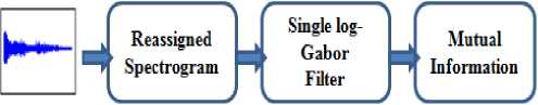
Fig.1. Feature extraction using single log-Gabor filter

• •    12 log-Gabor Filters concatenation applied to reassigned spectrogram

In this method, we tested log-Gabor filters for different concatenation numbers of log-Gabor filters N ^- = 2,3,4, ...,20 the best result is obtained for concatenation of 12 first log-Gabor filters that is for N ^- = 12.

In this method, each environmental sound reassigned spectrogram goes through a bank of 12 log-Gabor filters. This produces a bank of 12 log-Gabor filters {G _ii , G _i2 , ..., G _i6 , G ₂ i , -, G _{2 5} , G ₂₆ }, with each filter representing different scales and orientations. Thus, this result allows us to say that we obtain for each spectrogram a bank of 12 log-Gabor filters. These resulting feature values are later concatenated into 1D-vectors. Then the average computation is analysed according to the MI criteria, and is sent to SVM for classification (“Fig.2”).

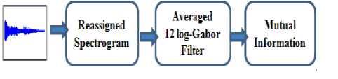
Fig.2. Feature extraction using 12 log- Gabor filters

• Three Reassigned Spectrogram Patches with 12 log-Gabor Filters

The method consists in using the reassigned spectrogram patch. The aim is to find the suitable part of spectrogram, where the efficient structure concentrates, which gives a better result. We tested our method using log-Gabor filter for three spectrogram patches. We tested for patch number Np = 2,3,4,5 , we remark that the satisfactory result is obtained for Np = 3.The idea is to extract three patches from each reassigned spectrogram. The first patch included frequencies from 0.01Hz to 128Hz, the second patch, from 128Hz to 256Hz, and the third patch, from 256Hz to 512Hz. Indeed, each patch goes through 12 log-Gabor filters, followed by an average operation and then, MI feature selection algorithm is used, which constitutes the parameter vector for the classification (“Fig.3”).

unseparable kernel allowing the spreads of the time and frequency smoothings bound, and even opposed [16], which leads to the spectrogram a loss of resolution and contrast [26].

Hence, the reassignment is going to re-focus the energy spread by the smoothing [23].

However, the reassignment application in time– frequency representation provides to run counter to its poor time-frequency concentration.

In this case the smoothing kernel ϕTF ( U , Ω) is the Wigner-Ville distribution of some unit energy analysis window ℎ( t ), with ϕTF ( и , Ω) = WV(ℎ; и ,Ω).

The values of the new position of energy contributions ( ̂( X ; t , 0) ), ω̂( X ; t , 0) )) are given by the center of gravity of the signal energy located in a bounded domain centered on ( t , 0) ) and measured by the Rihaczek distribution. These coordinates are defined by the smoothing kernel ϕTF ( и , Ω) and computed by means of short-time Fourier transforms in the following way [16]:

t̂(x;tω)=t- ^∫∫ . wv ( h ; , Я ) WV ( ; t-u , w-FZ )

;,            _∫∫wv(h; ,Я) WV( ;t-u,w-FZ) du^

=t-ℛ{

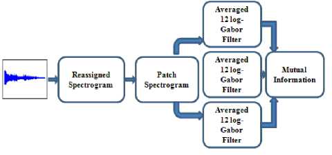
Fig.3. Feature extraction using 3spectrogram patches with 12 log-Gabor filters

∬ ․ Ri ∗₍ h ; , 41 ) Ri ( ; t-u , w-FZ ) du^ ∬ Ri∗(h; , 41 ) Ri ( ;t-u,w-FZ)du^

}

=t

_ ^ ( STFT_Th ( ;t , to). STFT ^∗ h( ;t, to )

-ℛ{      _|STFT_h (X;t, to)|        ^}

∫∫ 41 . WV ( h ; , 41 ) WV ( ; t-u , w-FZ ) du—

ω̂(x;t,ω)=ԝ-

∫∫WV(h; , 41) WV( ;t-u,w-FZ)du—

= ω

-ℛ{

∬ 41 ․ Ri ∗₍ h ; , 41 ) Ri ( ; t-u , w-FZ ) du^ ∬ Ri∗(h; , 41 )Ri( ;t-u,w-FZ)du^

}

=ω+

B. The Reassignment Method

The reassignment idea was presented first by Kodera et al. [3], then widens to the Cohen class of bilinear timefrequency energy distributions and to the refine class by Auger et al. and the affine smoothed pseudo Wigner-Ville distribution [17 16].

Besides, reassignment method allows the moving of the spectrogram values away from their computation place. In addition, it focuses energy components by moving each time-frequency location to its group delay and instantaneous frequency [23].

The spectrogram is the square modulus of the Short Time Fourier Transform STFTh (x; t, ω)

Sh(x; t, ω) =|STFTh(x; t, ω)|2          (1)

STFTh(x;t,ω)=∫  х(u)һ ^∗ (t - u)e -j_MU du  (2)

Moreover, the Time–frequency representation is more suitable and efficient for non-stationary signals.

Nevertheless, this representation has certain disadvantages. This disadvantage is manifested by its

Im{ STFT_Th( X ; t , to ).STFT ^∗ h ( ; t , to )

Im{       _|STFT_h (X;t, to)|         ^}

With Ri(x; t, ω) =x(t)․Х ^∗ (ω)e-jtot

where δ(t) is the Dirac impulse.

For more explication, you can see Appendix of [16]. The corresponding equation to the reassignment operators is writing in the following way:

MS_h = ∬ Sh ( x ; t ,w) 5 ( t' - ̂( x ; t ,w)). 5 ( w' -

̂( X ; t ,w)) ^dt5                                 (9)

According to [16] this reassigned version is also nonnegative, and retains all the properties of the spectrogram except the bilinearity, still lost for the benefit of perfectly localized chirps and impulses.

Furthermore, the time and frequency corrections expressions (5) and (8) lead to a reliable computation of the reassignment operators.

We adopted in this work the reassignment method in order to obtain a clear and easily interpreted spectrogram.

C. Log-Gabor filters

Gabor filters offer an excellent simultaneous localization of spatial and frequency information [20]. They have many useful and important properties, in particular the capacity to decompose an image into its underlying dominant spectro-temporal components [17].

The log-Gabor filters coefficients contain relevant and effective information. The robustness of the proposed feature is explained by the fact that log-Gabor filters consist in signal decomposition into spectro- temporal atoms, which are efficient to form an approximate representation.The log-Gabor function in the frequency domain can be described by the transfer function G ( г , 6 ) with polar coordinates [20]:

G(r,θ)=Gradial(r). Gangular (r)         (10)

Where ^radial ( r )=_e-!°g ⁽ r ^⁄ fo )⁄ 20? , is the frequency response of the radial component and ^angular ( T )= exp (-( 6 ⁄0_O )² ⁄2 ^e ), represents the frequency response of the angular filter component.

We note that ( r , 6 ) are the polar coordinates, /о represents the central filter frequency, 0_O is the orientation angle, a_r and a_e represent the scale bandwidth and angular bandwidth respectively.

The log-Gabor feature representation | S(x,У)| , of a magnitude spectrogram s(X,У) was calculated as a convolution operation performed separately for the real and imaginary part of the log-Gabor filters:

Re(S(x, y))m,n =s(x, y) ∗Re(G(rm,θn))

Im(S(x, y))m,n=s(x, y) ∗Im(G(rm,θn))

(X,У ) represent the time and frequency coordinates of a spectrogram, and m=1,…,NT=2 andn=1,…,=

6 where N_T devotes the scale number and Ng the orientation number. This was followed by the magnitude calculation for the filter bank outputs:

|S(x, y)|=√(Re(S(x, y))) +Im(S(x, y))m,n

• D.    Averaging outputs of log-Gabor filters

The averaged operation was calculated for each 12 log-Gabor filter appropriate for each reassigned spectrogram; the purpose being to obtain a single output array [20]:

|S ^̂ (x, y)|=       ^{∑  ,} :1⁶|S(x, y)| m , n        (14)

n=1

• E.    Mutual information

The information found commonly in two random variables is defined as the mutual information between two variables X and Y, and it is given as [27]:

I(Х;Y)=∑ ∈ x^∑ у ∈ Yр(x,y)log   ^{( , )}       (15)

()()

Where p ( X )= Pr ( X = ) is the marginal probability density function and p ( x )= Pr ( X = ) , and p ( x , У )= Pr ( X = , Y = ) is the joint probability density function.

• F.    SVM Classification

For the classification, we used a Support Vector Machine, in a One-against-One configuration. The SVM’s is a tool for creating practical algorithms for estimating multidimensional functions [28].

In the nonlinear case, the idea is to use a kernel function К ( X[ , Xj ), where К ( X[ , Xj ) satisfies the Mercer conditions [29]. Here, we used a Gaussian RBF kernel whose formula is:

• k(x i ,x j )=exp[ ‖ ^‖ ] (16)

We hence adopted one approach of multiclass classification: One-against-One. This approach consists in creating a binary classification of each possible combination of classes, and the result for к classes is к ( к - 1)/2. The classification is then carried out in accordance with the majority voting scheme [31].

• III. Environmental Sound Classification System based on Reassignment Method and Log-Gabor

Filters

• A.    Database Description

The corpus sound samples used in the sound recognition experiments derived from different sound libraries available [32-33]. In addition, using several sound collections is important and very necessary to create a representative, large, and enough diverse databases.

Among the sounds of the corpus we find: explosions, broken glass, door slamming, gunshot, etc. This database includes impulsive and harmonic sounds for example phone rings (Pr) and children voices (Cv). We used 10 classes of environmental sounds as shown in Table 1. All signals have a resolution of 16 bits and a sampling frequency of 44100 Hz that is characterized by a good temporal resolution and a wide frequency band, which are both necessary to cover harmonic as well as impulsive sounds. When building database, great care was dedicated to the selection of the signals. Indeed, when a rather general use of the classification system is needed, some kind of intraclass diversity in the signal properties should be existed in the database. Besides, the chosen sound classes are given in Table 1, and they are integrally of surveillance applications.

We indicate also that the number of items in each class is intentionally not equal, and sometimes very different.

Furthermore, an efficient and suitable surveillance system should be able to correctly recognize these sounds with a view to lower the false alarm rate. In addition, we remark in this database the presence of some classes sound very similar to human listeners such as explosions (Ep) are pretty similar to gunshots (Gs), hence, it is sometimes not obvious to discriminate between them. They are deliberately differentiated to test capacity of the system in separating very similar classes of sounds.

A type of sounds is required by the application, sounds are non-still, mainly of short durations, mainly impulsive audio signals, and presenting a big diversity intra-classes and a lot of similarity inter-classes. Most of the impulsive signals introduced into the base have duration of 1s, but some sounds possess much superior durations which can achieve 6s (for certain samples of explosions and the Human screams).

Table1. Classes of sounds and number of samples in the database used for performance evaluation

Classes	Train	Test	Total
Door slams (Ds)	208	104	312
Explosions (Ep)	38	18	56
Glass breaking (Gb)	38	18	56
Dog barks (Db)	32	16	48
Phone rings (Pr)	32	16	48
Children voices (Cv)	54	26	80
Gunshots (Gs)	150	74	224
Human screams (Hs)	48	24	72
Machines (Mc)	38	18	56
Cymbals (Cy)	32	16	48
Total	670	330	1000

“Fig.4”depicts environmental sounds spectrograms and their reassigned representation. Each class contains sounds with very different temporal or spectral characteristics, levels, duration, and time alignment. For example door slams (Ds) present a wide frequency band but with a short duration. In addition, for the children voices (Cv), we can distinguish the presence of the privilege frequencies. Concerning phone rings (Pr), we notice that they present fundamental frequencies. Furthermore, we notice that there are some similarities between explosions (Ep) and gunshots (Gs) although they belong to different classes. The used system should be able to discriminate sounds from these classes. Moreover, some used sounds present important energy content in the highest frequencies, for example glass breaking. Concerning the reassigned spectrogram as shown in figure 4, we notice a significant improvement in localization of the reassigned spectrogram in timefrequency domain in comparison to the spectrogram obtained by Short Time Fourier Transform. We can deduce that the reassignment method provides almost ideal representation of the environmental sound. We remark that the reassigned spectrogram provides good concentration at lower frequencies, but poor concentration at higher frequencies. In other words, the reassigned spectrogram obtained by the Short Time Fourier transform (STFT) enhances the concentration of the components in comparison to the spectrogram, and it does not contain any cross terms as shown in Figure 4 [34]. In addition, for reassignment spectrogram, we use the smoothing hanning window of length 256 with 192-point overlap. In order to obtain reassigned spectrogram it is necessary to compute auxiliary spectra and timefrequency corrections using the reassignment method of Auger and Flandrin previously described.

. e' Spectrogram Gunshots                         .id" Spectrogram Explosion

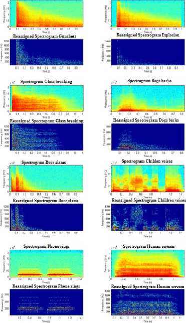
Fig.4. Spectrograms and their reassigned representation of 8 environmental sound classes

• B.    SVM Classifier Design and Parameters Setting

The SVM classifier design is previously described in Section 2. Thus, for multiclass classification, we evaluated the multiclass SVM (M-SVM) classifier One-against-One learn to discriminate one class from another.

Furthermore, One-against-One classifiers are generally smaller and can be estimated using fewer resources than One-against-All classifiers. In the classification context with SVM many studies like [35], proved that One-against-One classifiers are marginally more accurate than One-against-All classifiers. Hence, in this work we used One-against-One simply because is more suitable for practical use [31], and its training time is shorter than One-against-All. Most of the signals are impulsive.

We took 2/3 for the training and 1/3 for the test. Among the big problems met during the classification by the SVM’s is the choice of the values of the kernel parameter γ and the constant of regularization C . To resolve this problem we suggest the cross-validation procedure [36].

Indeed, according to [37], this method consists in setting up a grid-search for γ and C . For the implementation of this grid, it is necessary to proceed iteratively, by creating a couple of values γ and C.

The radial basis kernel was adopted for all the experiments. The parameter C was used also to determine the trade-off between margin maximization and training error minimization [38].

For the implementation of this grid, it is necessary to proceed iteratively, by creating a couple of values у and C. In this work, we use the following couples:

C , y: C [2 ( 5) , 2"^;i ,_. 2⁽¹⁵⁾] et у =[2^(-15), 2^(-14), ..., 2⁽³⁾].

The number of support vectors of our sound classes ranges between(45, ... ,89).

• C.    Experimental Results

• •    Results with Individual log-Gabor-filter

The results of the first method are summarized in Table 2, the classification rates for each single log-Gabor filter derived from reassigned spectrogram, which included 2 scales and 6 orientations, are relatively low, ranging from 51.78 to 99.35% for 10 sounds class.

The best classification result based on the first method belongs to the Door slams class with scale=1, and orientation=1 which is of the order 99.35%.

In addition, we achieved an averaged recognition rate of order 81.94%.

The reassignment method brings a good localization in time-frequency domain which ensures a high energy concentration. In order to improve the first method result, features should be extracted either from all log-Gabor filters or from a selected group of best performing filters [20].

Both the second and the third method are concentrated to improve and correct failures of first method.

• •    Results with Concatenation of the 12 log-Gabor-filters

In order to enlight the usefulness of the features presented in first method, we present classification results obtained when applying the concatenation of the 12 log-Gabor-filters to reassigned spectrogram in the feature vector.

Results of the second approach are illustrated in Table3. The obtained classification rate ranges from 85.71 % to 95.83. We were able to achieve an averaged accuracy rate of the order 92.07% in ten classes with one-against-one approach.

Furthermore, this method leads to an increase approximately 10 % of averaged recognition compared to the averaged result when we used single log Gabor filter method (81.94%).

We can deduce that the concatenation of 12 log-Gabor filters contains and concentrates the useful information than single log-Gabor filter.

Table.2 Recognition Rates of 12 log-Gabor filters applied to one-against-one SVM’s based classifier with Gaussian RBF kernel

Scale	Orienta-tion	Ds	Ep	Gb	Db	Pr	Cv	Gs	Hs	Mc	Cy
1	1	99,35	62.50	57.14	83.33	68.75	78.57	89.28	92.64	80.35	93.75
	2	96.15	55.35	60.71	79.16	70.83	82.14	89.73	89.70	82.14	89.58
	3	95.83	62.50	66.07	83.33	72.91	83.92	93.30	95.58	89.28	93.75
	4	99.03	55.35	67.85	81.25	81.25	78.57	88.39	92.64	78.57	85.41
	5	98.39	62.50	51.78	79.16	75.00	83.92	86.16	86.76	76.78	83.33
	6	99.03	58.92	51.78	81.25	79.16	81.25	85.71	86.76	80.35	83.33
2	1	95.83	62.50	71.42	87.50	87.50	89.28	95.83	89.70	92.64	93.75
	2	95.83	85.71	75.00	89.58	85.41	88.75	96.42	92.64	87.50	85.41
	3	80.12	64.28	88.75	93.75	87.50	85.71	95.08	95.58	85.71	95.58
	4	83.01	64.28	75.00	79.16	81.25	82.14	89.73	85.29	82.14	83.33
	5	80.44	64.28	67.85	77.08	79.16	83.92	93.30	92.64	83.92	85.41
	6	81.08	58.92	66.07	77.08	75.00	82.14	89.73	88.23	78.57	85.41

Table.3 Recognition Rates for averaged outputs of Reassigned Spectrogram with 12 log-Gabor filters, 3 Reassigned Spectrogram patches applied to one-against-one SVM’s based classifier with Gaussian RBF kernel

	Reassigned Spectrogram with 12 log-Gabor filters concatenation		3 Reassigned Spectrogram patches
Classes	ParametersKernel ( c, y)	Classif. Rate (%)	Parameters Kernel ( c, y)	Classif. Rate (%)
Ds	(2 (-1), 2 (-6) )	95.83	(2 (-5), 2 (-6) )	94.87
Ep	(2 (-1), 2 (2) )	85.71	(2 (-4), 2 (-6) )	88.75
Cb	(2 (2), 2 (3) )	91.07	(2 (-5), 2 (2) )	78.57
Db	(2 (-3), 2 (-14) )	93.75	(2 (1), 2 (3) )	89.58
Pr	(2 (-3), 2 (-7) )	93.75	(2 (15), 2 (1) )	93.75
Cv	(2 (-4), 2 (2) )	88.75	(2 (-1), 2 (-6) )	85.71
Gs	(2 (10), 2 (-5) )	93.30	(2 (-4), 2 (2) )	95.83
Hs	(2 (-1), 2 (-6) )	95.58	(2 (-3), 2 (-4) )	95.58
Mc	(2 (10), 2 (-1) )	89.28	(2 (-4), 2 (-6) )	92.85
Cy	(2 (-5), 2 (2) )	93.75	(2 (-3), 2 (-7) )	93.30

• •    Results with 12 log-Gabor-filters applied to the three patch reassigned spectrogram

Results of third approach are shown in Table 3. Besides, we obtained in this approach an averaged accuracy rate of the order 90.87%.This result is better than the first method result but is slightly lower than the second method result. Also, this method leads to an increase approximately 11% of averaged recognition compared to the result obtained when we applied single log-Gabor filters.

• •    Comments and Discussion

The reassignment method depends on the proper choice of smoothing kernel in order to produce simultaneously a high concentration of the signal components [16]. It permits to build a readable timefrequency representation process.

Moreover, the use of reassignment approach ensures an easily interpretation of spectrogram signature.

Nevertheless, previous studies [23-24-25] show that using reassignment method can improve the detection, the additive sound modeling, the segmentation and the classification performance.

The reassignment method allows removing the signal interference refocuses and concentrates the useful information. In this case it ensures good time-frequency decomposition.

Moreover, the use of reassignment method and log-Gabor filters offer the best simultaneous localization of spatial and frequency information. Generally, log-Gabor filters don’t have DC component, which helps to improve the contrast of the reassigned spectrogram. In addition, the transfer function of the Log-Gabor function has an extended tail at the high frequency end, which allows us to achieve wide spectral information with localized spatial extent [39].

Besides, SVMs have proven to be robust in high dimensions. They are well founded mathematically to reach good generalization while keeping high classification accuracy.

The performance of the proposed classification system has been evaluated with SVMs by using a set of synthetic test signals. However, proposed methods maintain overall good performance.

The experiments results are satisfactory, which encourages us to investigate better in the reassignment method.

• D.    Comparaison of state-of-the-art methods

In this section, our experimental result was compared to the state-of-the-art methods results. Table 5 illustrated different methods for environmental sounds recognition with their classification rate. We begin by the method tested in [40], which used acoustic features, the combination between 13 MFCCs, 1 RASTA-PLP, 5 Amplitude Descriptor (AD), 1 Spectral Flux (SF), 1 Loudness, has given an average classification rate of the order 88.2%. Then, in the work of D. Istrate et al. [9], which used as features 16 MFCCs+ energy+Д + ДД, the recognition rate is of the order 89.3%.

Furthermore, the studies of Chu et al. [1] proposed an approach based on combination of matching pursuit (MP) and MFCCs features. This combination gives the average classification rate of 83.9 % in discriminating fourteen classes with GMM classifier.

When comparing these previous methods results with our classification system, we remark that our system has significant and better results. The experimental results listed in Table 4 demonstrate our efficient features for environmental sound recognition. Our classification rate is of the order 92.07% when we used reassigned spectrogram with 12 log-Gabor filter concatenation.

To conclude, we compared also our obtained results with the results obtained by Rabaoui et al.[2], who used a combination between MFCCs, energy, Log energy, SRF (SpectralRoll-Off-Point and SC (Spectral Centroide). This method has given an average classification rate of (90.64%)

in the nine environmental sounds classes. With the same nine sounds classes (Door slams (Ds), Explosions (Ep), Glass breaking (Gb), Dog barks (Db), Phone rings (Pr), Children voices (Cv), Gunshots (Gs), Human screams (Hs), Machines (Mc)), and using 12 log-Gabor filters concatenation our recognition accuracy is of the order (91.89%). Our result shows that our features are significantly better in spite of their limited number. This can be partly explained by the fact that log-Gabor filters and reassignment method have the advantage of the best simultaneous localization of spatial and frequency information.

Nevertheless, as shown in Table 4, the classical method used various audio features combination, with selection criteria but here we opened a new research area using reassigned spectrogram as image texture for everyday sounds classification.

As can be seen in Table 4, our adopted features lead to an important improvement of the recognition accuracy when compared with the result done by classical features. According to the experimental results, our methods achieved enhanced performances in the visual domain.

Table.4 Comparison of state-of-the-art methods

Features	Classification Rate
13 MFCCs , 1 RASTA-PLP, 5 Amplitude Descriptor (AD), 1 Spectral Flux (SF), 1 Loudness [40]	88.2%
16 MFCCs+energy+A + ДД [9]	89.3%
Matching Pursuit (MP) + MFCCs [1]	83.14%
MFCCs+energy+Log energy+SRF(SpectralRoll-Off-Point+SC(Spectral Centroide) [2]	90.64%
Adopted Descriptors using 12 log-Gabor filters	92.07%

The adjustment of the visual features extraction methods used in image processing to the special characteristics of the environmental sounds have given satisfactory and improved classification results. Using reassignmen method, log-Gabor filters, a supervised method of classification (SVM) and a mutual information [41] gives the best discrimination between specific sound classes (92.07%).

• V. Conclusion

In this paper, a robust approach for improving the energy concentration of signals in the time-frequency domain has been proposed and tested to three new methods for environmental sound classification. This approach is based on the idea of reassigning the timefrequency representation of signal in order to obtain sharper representation.

We focused on novel sets of relevant features based on reassigned spectrogram. All methods used spectro-temporal components derived from log-Gabor filters. The first method uses a single log-Gabor filter. The second method uses an average of 12 log-Gabor filters concatenation. The third method segmented reassigned spectrogram into three patches with average of 12 log-Gabor filters. The two last methods showed promising results in the process of surveillance applications in the environmental sounds.

Our obtained results proved that the reassignment method is very efficient and it can be applied to a wide class of time frequency distributions.

In addition, this paper deals with robust features used with one-against-one SVM-based classifier in order to have a system that quietly works, independent of recording conditions. In all methods, the average highest classification accuracy was achieved while using the reassigned spectrogram with 12 log-Gabor filters concatenation (92.07%).

Future research directions will include other methods extracted from image processing to apply in environmental sound classification.