Opportunities to promote economic growth in Russia at a rate not lower than the world average

In recent years, the relevance and impact of research aimed at finding opportunities to promote economic growth in Russia on the basis of optimal relations between the factors of production have increased significantly both from the standpoint of the theoretical economy and from the standpoint of management practice. Thus, the use of real statistical data and correlations provides the basis for the natural development of fundamental concepts that formalize the mechanisms of economic growth. From the standpoint of management practice, the importance of assessing the opportunities and problems of economic growth within the existing structure of the economy is determined by at least two factors. First, it is the obvious necessity to address daily issues of economic growth, requiring the use of reliable and unambiguous tools of macroeconomic estimates, suitable for use in forecasting purposes. The second factor consists in a significant change in the official assessments of the country’s socioeconomic development prospects outlined in the Presidential decree of May 7, 2018 (Decree 204 “On national goals and strategic objectives for the development of the Russian Federation for the period up to 2024”, the so-called “May decree”). Thus, by 2024, the Government is to ensure the achievement of the following goals: “the Russian Federation is among the five largest economies in the world, Russia’s economic growth is above the world indicators, and its macroeconomic stability is preserved”. At the same time, we agree with V. Mau’s statement that “if earlier the economic forecasts of the Government were more like contingency plans, and included desirable (and sometimes fantastic) development scenarios, then since the fall of 2013, the official forecast started to proceed mainly from the extrapolation of existing trends...” [1]. Indeed, the Ministry of Economic Development of the Russian Federation updated the forecast of socioeconomic development in 2018, taking into account the goals set by the President of the Russian Federation in the May decree. The updated forecast considers the prerequisites for accelerating economic growth through a set of measures based on the increase in the factors of production – capital (increase in investment costs) and labor (increase in the number of people employed in the economy, including the increase due to the pension reform). However, it is difficult to assess the effectiveness of the proposed measures due to the apparent lack of theoretical substantiation for solving the problems of growth, including the assessment of the relationship between macroeconomic indicators, and factors of GDP production in relation to the Russian economy.

On the surface of quite a significant amount of fundamental and practical works, this insufficiency is manifested not only in diversity, but also in extreme assessments of the problems, opportunities and prospects of economic growth of the Russian Federation [2, 3, 4, 5]. Thus, the need to make a convincing assessment of the growth of the Russian economy indicates the necessity to apply strategies and techniques that will help assess the situation to select the correct model and the means of achieving strategic indicators corresponding to the specific realities. Such an approach exists in the vast majority of foreign works on growth models [6, 7, 8], in contrast to some Russian works that substantiate the development of the Russian economy without a detailed quantitative analysis.

The goal of the study is to assess the possibility of ensuring economic growth in Russia at a rate higher than the world average; the assessment is based on the study of optimal ratios of the factors of production of Russia’s GDP.

It should be noted that so far there are no such estimates; consequently, this fact determines fundamental novelty of our research estimated through the identification of stable relations and trends of economic growth in Russia; it also determines obvious scientific and practical novelty of our research.

Theoretical and methodological basis and the content of the research

Let us substantiate the content of the research, which is determined by the capabilities and limitations of modern theoretical and methodological tools on the profile of the study under consideration.

Theoretical and methodological foundations of objective estimates of economic growth based on the use of real statistics data suggest that production should be formalized through the functional relationship between the factors of labor and capital [9, 10]. Accordingly, by using classical fundamental concepts [11, 12, 13] confirmed by modern research [14, 15, 16], we rely on the generally accepted premise that labor and capital are the key elements of management necessary to stimulate or establish the further trajectory of economic growth. At the same time, numerous studies argue that specific economies characterize certain optimal ratios of the factors of production, which are relatively constant [17, 18, 19, 20]. That is, production functions allow us to consider the economic essence of production. We believe that this is the reason for the universality of the use of production functions in the practical tasks of managing macroeconomic processes. Production functions are included in the basic tools for forecasting and planning macroeconomic indicators of countries and regions of the world (forecast of the economy of Japan, USA, Canada, IMF ( World Economic Outlook ), UN ( World Economic Situation and Prospects ), etc.) [21].

As part of this approach, we propose a decomposition of the output (Russia’s GDP) and consider the relationship between the growth rates of volume indicators of resource costs.

Using the recent results of studies of the specifics of GDP and GRP production in Russia [21, 22], we will use the relationship between the factors of production (GDP and investment), normalized by the number of employees, reduced to the Cobb–Douglas production function [11]. This approach allows us to consider the relationship between the growth rates of specific indicators that link the value of total output to labor and capital costs, and then to define and select optimal ratios of the factors of production. Finally, we not only substantiate the optimal ratios, but also reflect their compliance with the real processes of production of Russia’s GDP. This makes it possible to identify fundamental problems and reveal actual opportunities for economic growth within the framework of the current economic model. It should be noted that the forecast nature of the estimates determines the need to take into account the impact of the pension reform. In order to find out what growth rates of investment in fixed capital are necessary to ensure the targeted GDP growth, taking into account the existing demographic constraints, we build a model of a multiplicative production function that connects the physical volume of GDP with investment in fixed capital.

The advantages of the research scheme we propose are as follows: first, the mathematical justification of the corresponding statements within the capabilities of modern methods and statistical base; second, the assessment of their compliance with real processes.

Input data and GDP production model

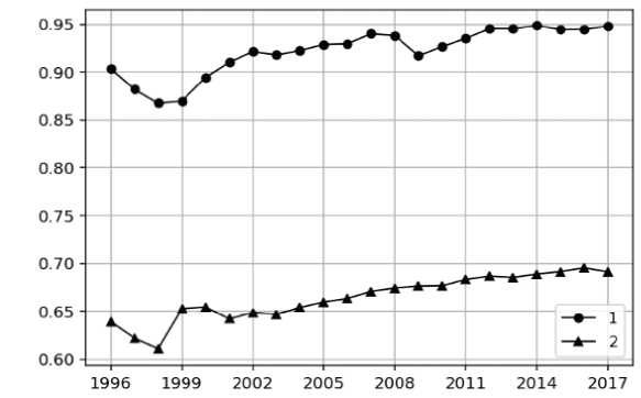
The study used the following data of the Federal State Statistics Service: indices of physical volume of GDP as a percentage of the previous year; investment in fixed capital in the Russian Federation at comparable prices as a percentage of the previous year; the number of people employed in the economy. The values of the indicators relative to the year 1995 are shown in Figure 1 .

Let us consider the ratio of GDP to the number of people employed in the economy and the ratio of investment in fixed capital to the number of people employed in the economy for 1996–2017 (22 observations). The correlation coefficient between these values is 0.989, so there is a statistically significant linear relationship: the observed value of the F -test (894) is greater than the

Figure 1. Physical volume of GDP (1), investment in fixed capital (2), and the number of persons employed (3) for 1996–2017 (data are shown relative to 1995)

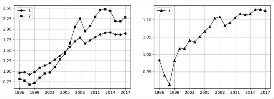
Sources: our own calculations with the use of Rosstat data.

Indices of the physical volume of GDP in % to the previous year for 1996–2017. Available at: new_site/vvp/vvp-god/ (accessed August 8, 2018); Investments in fixed capital in the Russian Federation in comparable prices in % to the previous year for 1995–2017. Available at: invest/ (accessed August 8, 2018); the number of employed in the economy in 1995–2016. Available at: (accessed August 8, 2018); 2017. Available at: indicator/58713 (accessed August 8, 2018).

corresponding table value (8.096) at 1% significance level. And therefore, a significant linear relationship is present between the logarithms of these relations (correlation coefficient is 0.993), which has the following form:

Ln( Y / L ) = p ln( K / L ) + a , (1)

where Y is GDP; K is capital, investment in fixed assets; L is labor, the number of people employed; p and a are regression parameters.

The formula (1) defines the relationship between output and investment normalized by employment. Expressing Y from the ratio (1), we obtain the following:

Y = AK ^pL ^q, p + q = 1. (2)

The expression (2) is a Cobb–Douglas production function (PF) [11], where A =exp( a ) is neutral technological progress, p is capital elasticity coefficient (fixed capital investment), q = 1 - p is labor elasticity coefficient (number of people employed).

Traditionally, the Cobb-Douglas function uses the value of fixed assets as capital K [11, 23]. However, in this case, the correlation coefficient between the logarithms of relations is 0.62, and its square is 0.38, that is, only 38% of the spread of the original data is determined by the model, so this model does not correspond to the original data. This feature of the production processes in the Russian economy is noted in a number of studies [21].

In this case, the use of the model in the form of a multiplicative PF Y = AK ^pL ^q (there is no condition p + q = 1, which determines the normalization on the number of employees) is unjustified. The reason is the presence of a significant correlation between investment K and the number of people employed L (correlation coefficient is 0.923).

The coefficient of elasticity determines the impact of changes in the resource used in production on the volume of output. For example, if capital ( K ) in (2) changes in x times, then GDP will change in x^p times. In order to

Figure 2. Comparison of actual and calculated according to the model (2) values of the index of physical volume of GRP in 1996–2017 relative to the year 1995.

R² – coefficient of determination. The black line is the line of the best match.

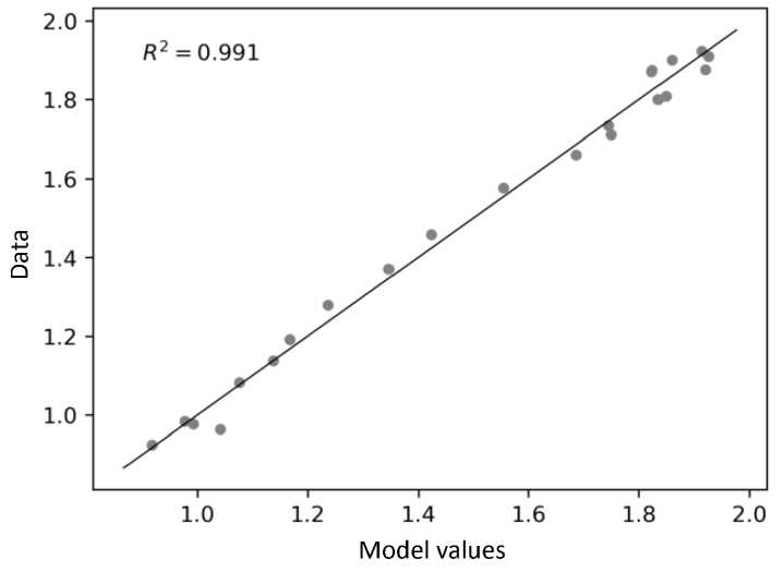
Source: our own calculations.

move to the elasticities we took the logarithm of the values of GDP and investment in fixed capital per person employed.

The results of model parameters estimation (2) are given in Table 1. The estimation was carried out by the least squares method according to the data for 1996–2017 (22 observations); the indicators were adjusted to the indices of physical volume relative to 1995 (Fig. 1) .

The model has a high determination coefficient R² = 0.991, which indicates the presence of a good correlation between the model and the initial data (Fig. 2) . The estimated capital ( p ) and labor ( q ) elasticities are within the range of 0 to 1 (Tab. 1). It means that: 1) with the increase in resources (capital and labor), GDP output also grows; 2) with the growth of resources, the growth rate of output slows down [24]. The coincidence of elasticities p = q = 0.5 shows that GDP production is equally determined by the number of employees and investments in fixed capital (the contribution of these indicators is the same).

Table 1. Values of parameters of the model (2) based on 95% confidence intervals, coefficient of determination

R² , estimated according to the data for 1996–2017

A	p	q	R2
1.160 ± 0.017	0.500 ± 0.03	0.500 ± 0.03	0.991
Source: our own calculations.

Search for optimal relations between labor and capital

While maintaining the structure of the economy, according to the model (2), in order to increase GDP it is necessary to increase investment in fixed capital and the number of employees. The same GDP growth can be achieved with different values of these factors.

Suppose it is necessary to increase GDP in r times, then, according to (2), we have: Yr = A(KrK) p (LrL) q, where the multipliers rK, rL show how many times you need to increase capital and labor, respectively, to ensure GDP growth in r times. Dividing this ratio by the expression (2), we obtain the following ratio:

r = r_K^p r_L^q , p + q = 1. (3)

Formally, the required GDP growth can be achieved in an infinite number of ways by changing r_K , r_L along the corresponding line of the function level (3). Under the optimal way we understand the way in which the ratio between the increase in capital and increase in labor provides the highest growth rate of the function (3). The desired ratio is determined by the gradient of the function (3) G = ( G_K , G_L ), whose components have the form:

G_K = p r_K^{p -1} r_L^q , G_L = r_K^p q r_L^{q -1}. (4)

The gradient (4) is perpendicular to the tangent lines of the level of the function r (3) at the corresponding points.

Thus, changing the values of r_K , r_L from the starting point r_K = r_L = 1 in the direction of the gradient at this point G = ( p , q ), we get the maximum possible rate of GDP growth:

r_K = 1 + sp , r_L = 1 + sq , (5)

where p and q are labor and capital elasticity coefficients, respectively; the factor s is determined for the required GDP growth r from the equation (3) by substituting the expressions (5) into it. Assuming that p = q = 0.5 (Tab. 1), we obtain s = 2 r – 2. Substituting this expression in (5), we obtain:

r_K = r_L = r . (6)

To ensure the growth of Russia’s GDP in r times the best way, it is necessary to increase the number of people employed and investment in fixed capital in the same r times . This is the main result of the present study.

Note that the formula (6) is valid only if p = q = 0.5. For other values of elasticity p and q in order to find s , the equation (3) is solved numerically for the given GDP growth r by substituting the expressions (5) into it.

According to the decree of the President of the Russian Federation “On national goals and strategic objectives for the development of the Russian Federation for the period up to 2024” dated May 7, 2018, it is planned “to ensure that the Russian Federation will be among the five largest economies in the world, that its economic growth rates will be above the world average while its macroeconomic stability is maintained, and inflation remains at a level not exceeding 4%”. According to the World Bank, average global GDP growth rate in 2010–2017 was about 3% per year (Fig. 3) . To ensure the growth of Russia’s GDP by 3% per year ( r = 1.03) in the optimal way, according to the formula (6), it is necessary to increase investments in fixed capital and the number of employees by 3% annually.

Figure 3. World GDP for 2010–2017 (trillion USD) in 2010 prices (at an average growth rate of 3% per year)

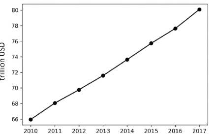
Source: compiled with the use of World Bank data

Website of the World Bank. Available at: https://data. locations=1W (accessed August 8, 2018).

In general, if the number of employees will increase in r_L times, then to ensure GDP growth in r times, it follows from the ratio (3) that investment in fixed capital should be increased in r_K = r ^{1/ p} r_L ^{- q / p} times, at q = p = 0.5 we get r_K = r ²/ r_L times.

Discussion of the results

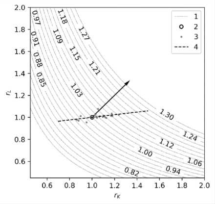
Figure 4 provides a graphical illustration that shows the following: level lines of the function (3) at the estimated values p = q = 0.5 (Tab. 1) corresponding to the different values of GDP growth; direction of the gradient (4) of the function (3) emerging from the starting point (1.1); actual capital and labor gains for 1996–2017 and the corresponding direct regression.

It is noteworthy that GDP growth during this period was achieved mainly due to an increase in investment rather than the number of employees. Indeed, against the background of the almost double GDP growth observed in 1998–2014, investment grew in 3.4 times and the number of people in employment – only in 1.13 times (Fig. 1). This phenomenon is also reflected in a significant deviation in the values of the growth of investment in fixed capital and the number of employees from the optimal direction set out by the gradient of the function (3) – the clockwise angle between the gradient and the actual regression is 38° (Fig. 3). The only exceptions are the years 1999 and 2002, when GDP growth ( r ) was achieved at the expense of approximately equal increases in fixed capital investment ( r_K ) and employment ( r_L ) relative to previous years. Thus, in 1999: r = 6.5%, r_K = 5,3%, r_L = 7.7% (the maximum value for 1996–2017); in 2002: r = 4.7%, r_K = 2,9%, r_L = 2.4%. In other years, GDP growth was mainly driven by increased investment.

Figure 4. Dependence of the increase in labor ( r_L ) and capital ( r_K ) corresponding to different values of GDP growth

• 1    – level lines of the function (3), captions correspond to the values of GDP growth r ;

• 2    – initial value of labor and capital gains – point (1.1). The arrow shows the direction of the gradient (4) of the function (3) that begins in the starting point (1.1);

• 3    – actual values of labor and capital gains for 1996–2017;

• 4    – trend line defined by the direct regression r_L = 0,119 r_K + 0.881 based on the actual data for 1996–2017 (the clockwise angle between the line 3 and the gradient is 38°).

Source: our own calculations.

In this case it is appropriate to raise the question of why GDP growth did not occur optimally. To answer this question, we compare the dynamics of the ratio of the labor force 15– 72 years of age to the number of employees, or (which is the same) 1 minus the unemployment rate (Fig. 5) with the dynamics of GDP growth (Fig. 1). Let us recall that labor force includes persons aged 15–72, who in the period under review are considered employed or unemployed.

For example, we take the ten-year period from 1999 to 2008, when GDP growth was the most stable. During this period, GDP grew by 83%, and the average growth rate was 7% per year. It turns out that with optimal GDP growth, the number of people employed and investment in fixed capital should have had the same average annual growth rate. That is, the ratio of the number of employees to the size of labor force in 2000 was to be 95.6%, and since 2001 (104%) and later on – more than 100%. By 2008, this ratio would have reached 170%. It is impossible to ensure such growth rate of the number of employees without increasing the level of participation in labor force (the ratio of the labor force of a certain age group to the total population of the corresponding age group; Fig. 5). That is why the average growth rate of investment in fixed assets for 1999–2008 was 13.4% per year, and average growth rate of the number of employees was 1.3% per year.

The issue concerning the size of labor force will arise even more acutely during the execution of the May 2018 decree, because, unlike the situation in 1999, the unemployment rate in the Russian Federation in 2017 was 5.2% (in 1999, it was greater – 13%).

Figure 5. Dynamics of the ratio of the number of employees to the size of labor force (1), and dynamics of labor force participation (the ratio of the labor force of a certain age group to the total population of the relevant age group) at the age of 15–72

Source: our own calculations.

Thus, in order to achieve optimal increase in GDP by 3% in 2018, according to the formula (6), the number of employees must also be increased by 3%. That is, the ratio of this indicator to the size of labor force will also increase by 3% compared to 2017 and will be 97.6% (unemployment is 2.4%). In 2019, the number of employees should be increased again by 3%, but relative to 2018. That is, the ratio of this indicator to labor force will increase by 3% (compared to 2019) and will be 100.5%. In order to ensure optimal employment growth, it is necessary to increase the level of participation in labor force, which is equivalent to a decrease in the number of economically inactive population, the share of which is more than 30% (Fig. 5).

According to the Rosstat classification of statistical data on the composition of labor force, economic activity and employment status [25], economically inactive population consists of six categories:

• a)    pupils, students, and cadets enrolled in intramural education programs (including intramural post-graduate studies);

• b)    persons who receive old-age and preferential pensions and those who receive survivor pensions when they reach retirement age;

• c)    persons who receive disability pensions (groups I, II, III);

• d)    persons engaged in housekeeping, childcare, care for sick relatives, etc.;

• e)    discouraged workers, i.e. persons who have given up on searching for a job because they have exhausted all the opportunities to get it, but they are eligible for employment and are able to work;

• f)    other persons who do not need to work, regardless of their source of income.

Only category “b” can be directly regulated. The planned increase in the retirement age [25] will reduce the number of this category by transferring some people either to labor force (employed or unemployed), or to the category “e” – “discouraged workers”. This conclusion points to the need to conduct a thorough study of the socio-economic consequences of the pension reform before its adoption, and the study should involve research teams, as well.

Thus, the increase in GDP in the Russian Federation under the current economic structure is possible mainly at the expense of the increase in investments. We note that a similar situation should be observed in other countries with low unemployment. The shortage of labor force is partly compensated for by the involvement of immigrants.

A model of increasing GDP with the help of increasing investments

In the final part of our study, we will answer the question about the possibility of increasing GDP only by increasing investments. To do this, we consider the relationship between GDP and investment.

The correlation between the physical volume of GDP relative to 1995 and investment in fixed capital in comparable prices relative to 1995 (Fig. 1) is 0.989. Reasoning in the same way as in the construction of the model (2), we obtain a ratio that is a multiplicative production function:

Y = A K ^p , (7)

where Y is GDP, K – investment in fixed capital; A and p (the coefficient of elasticity of investment) – parameters of the model.

The model (7) has a simple interpretation. The state regulates investments in fixed capital, and the required number of employees is determined on the basis of the existing institutional environment, current regulatory framework and economic situation.

The results of estimating the parameters of the model (7) are given in Table 2. The model has a high determination coefficient R2 = 0.987, which indicates a good correspondence of the model to the initial data (Fig. 6). The estimation of the value of capital elasticity p = 0.563 shows that in order to increase GDP in r times it is necessary to increase investment in rK = r1/p = r1.776 times (Fig. 7). Thus, to ensure GDP growth at the level of not less than 3% per year, as determined by the May 2018 decree, the increase in investment in fixed capital should be no less than 5.4% per year.

Table 2. Values of parameters of the model (7) based on 95% confidence intervals, determination coefficient R² , estimated according to the data for 1996–2017

A	p	R2
1.165 ± 0.02	0.563 ± 0.03	0.987
Source: our own calculations.

Figure 6. Comparison of the actual values of the index of GDP volume for 1996–2017 and those calculated according to the model (7) relative to 1995. R² -determination coefficient. The black line is the line of the best match.

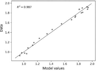
Source: our own calculations.

Figure 7. Increase in fixed capital investment r_K , calculated according to the model (7), required to increase GDP in r times

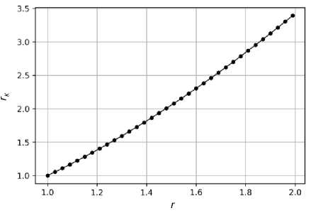
Source: our own calculations.

Conclusion

Consideration of the economic growth of Russia in the context of fundamental concepts by formalizing the mechanisms of economic development from the standpoint of determining the relationship and justification of optimal ratios of GDP production factors allowed us to obtain new theoretical knowledge. First, we substantiate the model of Russia’s GDP production, which expresses the functional relationship between the indices of the physical volume of GDP on the one hand, and the labor (number of employees in the Russian economy) and capital (investment in fixed capital) factors on the other. The model corresponds well to the initial statistical data: the coefficient of determination between the model and real data is more than 99%. Second, we substantiate the optimal ratio between investment and employment necessary to increase Russia’s GDP. Third, we carry out a detailed analysis of the correspondence of these optimal ratios to the real processes of GDP production. On this basis, we identify fundamental problems and possibilities of economic growth in the current economic model, taking into account the impact of the pension reform. We prove that the increase in GDP in Russia under the current economic structure is possible mainly due to the growth of investment. Fourth, on the basis of modeling (compliance of the constructed model with the initial data is good, the coefficient of determination is more than 98%), we consider the possibility of increasing Russia’s GDP with the help of investment. The assessment shows that in order to ensure GDP growth at the level of not less than 3% per year, which is set out in the May 2018 decree of the President, the growth of investments in the main capital should be at least 5.4% per year.

The development of theoretical concepts has provided valuable scientific and practical knowledge about the resources and limits of economic growth, management capabilities to ensure maximum efficiency of decisions, reduce the risks of management of the macroeconomic factors of production, and determine the investment conditions of economic growth.