Optimal Control for Industrial Sucrose Crystallization with Action Dependent Heuristic Dynamic Programming

Published Online October 2009 in MECS

The process of sucrose production consists mainly of press, clarification, evaporation, crystallization (sugar boiling). The sucrose crystallization incorporates both the heat and mass transfer, is the last and the most crucial step. The purpose of sugar boiling is to recover as much sugar from the syrup as possible, in the mean time; the size of the crystal should be as homogeneous as possible. The quality of the final product, the production efficiency and the economic benefits in sugar boiling technology were affected by the sucrose crystallization [14].

The super saturation (The degree to which the sucrose content in solution is greater than the sucrose content in saturated solution.) of sucrose solution is the key factor which impacts the sugar boiling process. We must keep

Manuscript received January 17, 2009; revised June 18, 2009; accepted July 28, 2009.

This work was supported by the Open Fund of Key Laboratory of Complex Systems and Intelligence Science, Institute of Automation, Chinese Academy of Sciences (20070101).

the super saturation in a metastable zone (keeping the super saturation in 1.20-1.25) to speed up the crystallization rate and ensure the quality of crystal [14]. So, how to ensure the stability of the super saturation is the key to sugar boiling automation. Approximate dynamic programming doesn’t need a precise mathematical model of the plant, can solve the optimization control problem of nonlinear system. In this paper, action dependent heuristic dynamic programming is used to optimize the sucrose crystallization by controlling the Brix of the sucrose solution based on a large number of Brix data from the actual sugar boiling process of sugar refinery. This is of great practical significance to improve the production efficiency of the sugar boiling process.

• II.    Approximate Dynamic Programming

• A.    Dynamic Programming for Discrete-Time Systems

Dynamic programming is a very useful tool in solving optimization and optimal control problems. It is based on the principle of optimality: An optimal policy has the property that whatever the initial state and initial decision are, the remaining decisions must constitute an optimal policy with regard to the state resulting from the first decision [1].

We can use mathematical language to express the principle of optimality above [11]. Suppose that one is given a discrete-time nonlinear dynamical system

x ( k + 1) = F [ x ( k ), u ( k ), k ] , k = 0,1,... .           (1)

where x e R ⁿ represents the state vector of the system and u e R m denotes the control action and F is the system function. Suppose that one associates with this system the performance index (or cost)

от

J [ x ( k ) , k ] = E Y" k U [ x ( i ) , u ( i ) , i J -          (2)

i=k where U is called the utility function and Y is the discount factor with 0 < у < 1. Note that the function J is dependent on the initial time k and the initial state x(k), and it is referred to as the cost-to-go of state x(k). The objective of the dynamic programming problem is to choose a control sequence u(i), i = k, k+1, …, so that the function J (i.e., the cost) in (2) is minimized.

Suppose that one has computed the optimal cost J * [ x ( k + 1), k ] from time k +1 to the terminal time, for all possible states x ( k +1), and that one has also found the optimal control sequences from time k +1 to the terminal time. The optimal cost results when the optimal control sequence u * ( k + 1), u * ( k + 2),..., is applied to the system with initial state x ( k +1). If one applies an arbitrary control u ( k ) at time k and then uses the known optimal control sequence from k +1 on, the resulting cost will be

U [ x ( k ), u ( k ), k ] + y J * [ x ( k + 1), k ]

where x ( k ) is the state at time k , and x ( k+ 1) is determined by (1). According to Bellman, the optimal cost from time k on is equal to

J * [ x ( k ), k ] = min { U [ x ( k ), u ( k ), k ] + y J * [ x ( k + 1), k ] } . (3)

The optimal control u ^* ( k ) at time k is the u ( k ) that achieves this minimum, i.e.,

u * ( k ) = argmin { U [ x ( k ), u ( k ), k ] + y J * [ x ( k + 1), k ] } . (4)

Equation (3) is the principle of optimality for discretetime systems. Its importance lies in the fact that it allows one to optimize over only one control vector at a time by working backward in time. In other words, any strategy of action that minimizes J in the short term will also minimizes the sum of U over all future times.

• B.    Basic Structure and Principle of ADP

Dynamic programming has been applied in different fields of engineering, operations research, economics, and so on for many years. It provides truly optimal solutions to nonlinear stochastic dynamic systems. However, it is well understood that for many important problems the computation costs of dynamic programming are very high, as a result of the “curse of dimensionality” [1].

Over the years, progress has been made to circumvent the “curse of dimensionality” by building a system, called “critic”, to approximate the cost function in dynamic programming [3], [4]. The idea is to approximate the dynamic programming solutions by using function approximation structures to approximate the optimal cost function and the optimal controller.

In 1977, Werbos introduced an approach for approximative dynamic programming that was later called adaptive critic designs (ACDs) [2]. ACDs were proposed in [2], [3] as a way for solving dynamic programming problems forward-in-time. ACDs have received increasing attention recently. In the literature, there are several synonyms used including “Adaptive Critic Designs” (ACDs), “Approximative Dynamic Programming”, “Adaptive Dynamic Programming”, and so on. The main idea of ADP is shown in Fig. 1 [13].

The whole structure consists of three parts: Dynamic System, Control/Action module, and Critic module. The Dynamic System is the plant to be controlled. The Control/Action module is used to approximate the optimal control strategy, and the Critic module is used to approximate the optimal performance index function. The combination of the Control/Action module and the Critic module is equivalent to an agent. After the Control/Action module acts on the Dynamic System (or the controlled plant), the Critic module is affected by a Reward/Penalty signal which is produced by environment (or the controlled plant) at various stages. The Control/Action module and the Critic module are function approximation structures such as neural networks. The parameters of the Critic module are updated based on the Bellman’s principle of optimality, and the objective of updating the parameters of the Control/Action module is to minimize the outputs of the Critic module. This not only minimizes the time of forward calculation, but also can online response dynamic changes of unknown system and adjusts some parameters of the network structure automatically. In this article, both the Control/Action module and the Critic module are neural networks, so they are also known as Control/Action network and Critic network.

• C.    Heuristic Dynamic Programming

In order to solve dynamic programming problems, various function approximation structures were proposed to approximate the optimal performance index function and the optimal strategy directly or indirectly.

Existing adaptive critic designs [5] can be categorized as: 1) heuristic dynamic programming (HDP); 2) dual heuristic programming (DHP); and 3) globalized dual heuristic programming (GDHP). One major difference between HDP and DHP is within the objective of the critic network. In HDP, the critic network outputs the estimate of J in (2) directly, while DHP estimates the derivative of J with respect to its input vector. GDHP is a combination of DHP and HDP, approximating both J ( x ( k )) and d J ( x ( k )) / d x ( k ) simultaneously with the critic network. Action dependent variants from these three basic design paradigms are also available. They are action

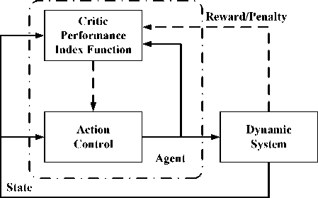
Figure 1. The structure of approximate dynamic programming [13].

dependent heuristic dynamic programming (ADHDP), action dependent dual heuristic programming (ADDHP), and action dependent globalized dual heuristic programming (ADGDHP). Action dependent (AD) refers to the fact that the action value is an additional input to the critic network.

HDP is the most basic and widely applied structure of ADP [6], [7], [8], [9]. A typical design of HDP controller consists of three networks: action network, model network and critic network. Each of these networks includes a feed-forward and a feedback component. The action network outputs the control signal, the model network simulates the characteristics of controlled object and outputs new state parameter, and the critic network outputs an estimate of cost function given by the Bellman equation associated with optimal control theory. The structure of HDP is shown in Fig. 2 [13].

In Fig. 2, the solid lines represent signal flow, while the dashed lines are the paths for parameter tuning. It will generate control signal u ( k ) when the action network accepts the system state x ( k ), then u ( k ) and x ( k ) add to the model network which will predict new state parameter x ( k+ 1), x ( k+ 1) is the only input parameter of the critic network which will output an approximate value of J function given by (2).

In HDP, the output of the critic network is J , which is the estimate of J in (2). This is done by minimizing the following error measure over time

II ^EA = £ Ec ( k )

k

A

A

= 1 £ J ( k ) - U ( k ) - y J ( k + 1) ² k -

where J ( k ) = J ( x ( k ), u ( k ), k , W C ) , W C represents the weights of the critic network. When E c ( k ) = 0 for all k , (5) implies that

J ( k ) = U ( k ) + y J ( k + 1)

= U ( k ) + y ( U ( k + 1) + y J ( k + 2))

which is exactly the same as the cost function in (2). It is therefore clear that minimizing the error function in (5), we will have a neural network trained so that its output J becomes an estimate of the cost function J defined in (2).

The aim of training the action network is minimizing the output of the critic network J . We seek to minimize

J in the immediate future thereby optimizing the overall cost expressed as a sum of all U( k ) over the horizon of the problem [5].

• D.    Action-Dependent Heuristic Dynamic Programming

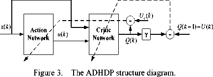
ADHDP is an Action-dependent form of HDP, its structure has only action network and critic network, as is shown in Fig. 3. One major difference between ADHDP and HDP is within the input of the critic network. In HDP, state variable is the only input of the critic network, while in ADHDP both state variable and control variable are the inputs of the critic network. In ADHDP, the output of critic network is usually known as Q -function which estimates the J function given by (2), so ADHDP is also known as Q -learning [10], [11], [12].

In ADHDP, there is no model network, and the action value is an additional input to the critic network. This gives us a few advantages including the simplification of the overall system design and the feasibility of the present approach to application where a model network may be very difficult to obtain [11]. In this article, we use ADHDP method to optimize the sucrose crystallization.

Critic Network : The critic network is used to provide Q as an approximation of J in (2). This is done by minimizing the following error measure over time.

E c = £ E c ( k ) = £ 1 e c ( k )² .         (7)

kk 2

where ec (k) = yQ(k) - (Q(k -1) - U(k)).         (8)

where Q(k) = Q[x(k), u (k), k, Wc ] and Wc represents the да

= £ y- ^kU ( i ) i = k

parameters of the critic network. The function U is the same utility function as the one in (2) which indicates the performance of the overall system. The function U given ⁽⁶⁾             in a problem is usually a function of x ( k ), u ( k ),

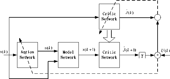
Figure 2. The HDP structure diagram [13].

and k , i.e., U ( k ) = U ( x ( k ), u ( k ), k ). When

E c ( k ) = 0 for all k , (7) implies that

Q ( k ) = U ( k + 1) + y Q ( k + 1)

= U ( k + 1) + y ( U ( k + 2) + y Q ( k + 2))

да

= £ y ' ^{- k}-1 U ( i )

i = k + 1

Clearly, comparing (2) and (9), we have now

Q ( k ) = J ( x ( k + 1), k + 1 ) . Therefore, when

minimizing the error function in (7), we have a neural

network trained so that its output becomes an estimate of the performance index function defined in (2) for i = k +1, i.e., the value of the performance index function in the immediate future.

The weights of the critic network are updated according to a gradient-descent algorithm

W_c ( k + 1) = W_c ( k ) + A W_c ( k ) .                 (10)

A W ( k ) = l ( k ) ^f- ^d E c ^{( k} ) )

^{c V} \ d w c ( k )J

( d E c ( k ) d Q ( k ) )

l ( k )

c ( d Q ( k ) d W c ( k ) J

where l c ( k )(0 <  l c ( k ) <  1) is the learning rate of the critic network at time k , which usually decreases with time to a small value, and W_c is the weight vector in the critic network.

Action Network: The principle in adapting the action network is to indirectly back-propagate the error between the desired ultimate objective, denoted by Uc , and the output of the critic network Q. Uc is set to “0” in our design paradigm and in our following case studies. The weight updating in the action network can be formulated as follows [10]. Let ea (k) = Q (k) - Uc (k). (12)

The weights in the action network are updated to minimize the following performance error measure

1 -

E a ( k ) = 2 ■ e a ²( k ).

The update algorithm is then similar to the one in the critic network. By a gradient descent rule

W a ( k + 1) = W a ( k ) + A W a ( k ).                  (14)

A W a = l a ( k )

d E a ( k ) )

5 W , ( k ) J

l _{( k} ) f ⁹ E a ( k ) d Q ( k ) d u ( k ) ) ^{a l} \ d q ( k ) d u ( k ) d W a ( k ) J . ₍₁₅₎

where l a ( k ) >  0 is the learning rate of the action network at time k , which usually decreases with time to a small value, and W_a is the weight vector in the action network.

• III.    Sucrose Crystallization

• A.    Formation of Sucrose Crystals

In sucrose solution, sucrose molecules distribute uniformly in the space of water molecules. Under the conditions of a certain concentration and temperature, the sucrose solution becomes saturated. The sucrose molecules steadily fill the space of water molecules, and achieve a balance combining with water molecules. When the number of sucrose molecules exceeds the inherent amounts of sucrose molecules in saturated solution, the balance will be broken, from balance to imbalance, stable to unstable. Even more, when the sucrose molecules reach a certain number, the distance between them lessens and the opportunity of collision increases. So the attraction between molecules gradually surpasses repulsion, and then some sucrose molecules can gather together, thus, sucrose crystals gradually form [14].

• B.    Sucrose Crystallization

At the beginning of crystallization, seeds usually with no uniform size. So we need to use water or syrup to dissolve part of small crystals and keep crystals homogeneous. This is called collation. After collation, the super saturation of syrup is relatively low in general, can not meet the requirement of the crystallization. At this time, the syrup needs to be enriched, the process known as enrichment A. When the syrup is enriched to a certain extent the crystal growth process start. It’s the main process of sucrose crystallization, accounting for the most of time for the crystallization. If improper operation occur in sucrose crystallization, pseudocrystals will appear. The pseudocrystals need to be washed away by water. If water injection rate is faster than evaporation rate, Brix of syrup will decline. So we need a water boiling process to make the super saturation return to the required value for crystallization. At the end of crystallization, we need to enrich massecuite (called enrichment B). When the massecuite is enriched to a certain extent, we can stop and complete the sugar boiling process [14].

• C.    Factors Which Affect Sucrose Crystallization

According to the analysis of sucrose crystallization and practical experience, we know that many factors affect the crystallization. These factors include the feed rate, the water inflow, the purity of the syrup, the vacuum of tank, the material temperature, the volume of sucrose solution, the heating steam pressure and temperature, and so on [14]. In this paper, we assume that the purity of the syrup is relatively stable for a period, and the super saturation of the syrup can also be kept in a relatively stable range. Under these assumptions, we study three key factors which impact the crystallization, i.e., the vacuum of tank, the heating steam pressure and temperature.

• D.    Neural Network Model of Sucrose Crystallization

In sucrose crystallization, Brix is proportional to supersaturation, and determines the crystallization rate. The neural network has strong nonlinear mapping (fitting)

characteristics [15]. In this paper, we developed a neural network model of the crystallization based on the data from the actual sugar boiling process of sugar refinery. We use the vacuum of the tank, the heating steam pressure and temperature as the inputs of the neural network, Brix degree as the output of the network. The neural network model is shown in Fig. 4.

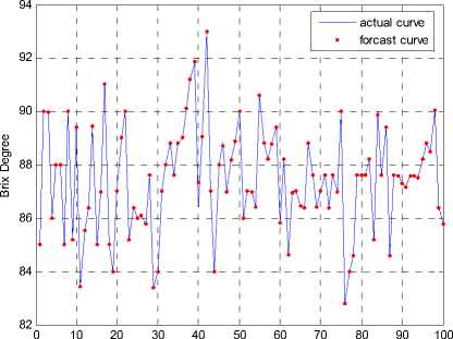
The data came from the actual production process of Liaoping Sugar Refinery of Guangxi. The neural network modeling mainly has several important links: data pretreatment, data normalization, network design, network training and network test, and so on. When processing the sample data, summarizing the operation range of sampled variables based on technical requirements and operation experiences, parts of the data can be primarily eliminated. After being processed, 500 sets of data are used as training samples, and 100 sets of data are used as testing samples, the data become numerical values between (-1,1) after a normalization process. Our designed neural network is chosen as a 365-1 structure with 3 input neutrons, 65 hidden neutrons and 1 output neutron. For this neural network, the hidden layer and output layer use the sigmoidal function tansig . We have applied trainlm (the Levenberg-Marquardt algorithm) for the training of the netwok. The trained model is shown in Fig. 5.

• IV.    The design of the controller

• A.    Control Objective of Brix and Sugar Boiling Time for Every Stage

According to the principle of sugar boiling process, statistical analysis of the sample data form actual production process of sugar refinery, and the practical experience of workers, we can get the control objective of Brix and the sugar boiling time for every stage, which is shown in Table I.

• B.    Defining of Utility Function

The definition of utility function is not exactly the same, because the control objectives of various stages are different. For example, we have need to control the Brix degree of the collation process in the scope of 82-86Bx, so the utility function is defined as

J ( % ( k ) - 84)2,| % ( k ) - 84| <  3

U ( k ) = |

[        1, otherwise                  (16)

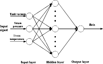
Figure 4. The neural network model for sucrose crystallization.

• C.    Design of Network and Algorithm Implementations

acquisition number

TABLE I.

the control objective of B rix and the sugar boiling time for EVERY STAGE

Stage	Control objective of Brix / Bx	Sugar boiling time / min
Collation	82--87	25
Enrichment A	88.2--90	25
Crystal Growth	88.2--90	120
Water Boiling	84--88	30
Enrichment B	92--94	20

Two BP neural networks are needed in the design of the ADHDP controller for sucrose crystallization, one is used as action network, and the other is used as critic network. In our ADHDP design, both the action network and the critic network are nonlinear multilayer feedforward networks. In our design, one hidden layer is used in each network. In the following, we devise learning algorithms and elaborate on how learning takes place in each of the two networks.

The critic network : The critic network is chosen as a 48-1 structure with 4 input neurons and 8 hidden layer neurons. The 4 inputs are the outputs of the action network u 1( k ), u 2( k ) and u 3( k ), and the Brix degree which is denoted by x ( k ). For the critic network, the hidden layer uses the sigmoidal function tansig , and the output layer uses the linear function purelin . The structure of the critic network is shown in Fig. 6.

There are two processes for training the network. One is the forward computation process and the other is the error backward propagation process which updates the weights of the critic network.

In the critic network, the output Q ( k ) will be of the form

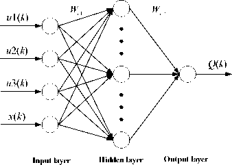
Figure 6. The structure of critic network.

heating steam pressure and the heating steam temperature respectively. Both the hidden layer and output layer use the sigmoidal function tansig . The neural network structure for the action network is shown in f ig . 7 .

Now, let us investigate the adaptation in the action network; the associated equations for the action network are ch1( k) = inputC (k) x Wc 1( k)

ah 1( k ) = x ( k ) x Wa 1 ( k ).	(24)
ah 2( k ) = tan sig ( ah 1( k )).	(25)
v ( k ) = ah 2( k ) x Wa 2 ( k ).	(26)
u ( k ) = tan sig ( v ( k )).	(27)

ch 2( k ) = tan sig ( ch1(k )) .               (18)

Q ( k ) = ch 2( k ) x W c ₂ ( k )

where inputC: input vector of the critic network, inputC=[u1 u1 u3 x];

ch 1: input vector of the hidden layer;

ch 2: output vector of the hidden layer;

By applying the chain rule, the adaptation of the critic network is summarized as follows.

1) W_{c 2} (weight vector for hidden to output layer)

W c ₂ ( k + 1) = W c ₂ ( k ) + A W c ₂ ( k )

where ah1: input vector of the hidden layer;

ah 2: output vector of the hidden layer;

• v : input vector of the output layer;

By applying the chain rule, the adaptation of the action network is summarized as follows.

• 1)    W_{a 2} (weight vector for hidden to output layer)

W a 2 ( k + 1) = W a 2 ( k ) +A W_Q 2 ( k ).                 (28)

a W ₂( k ) = l _a ( k ) f— ^E a ^kL ¹

a ² I d W_{a 2} ( k ) J

= | ( k ) f ^d E ° ^{( k} ) ⁸ Q ( k ) ^{8 u} ( k ) ⁸ v ( k ) )

^Л \ d Q ( k ) d u ( k ) d v ( k ) d W„ ₂ ( k ) J

A W ( k ) = l ( k ) ^f- ^d E c ^{( k} ) ) c ²¹ c ' \ d W c 2( k )J

_     ( d E c ( k ) d q ( k ) 1

l ( k )

c Я ⁵ Q ( k ) d W c 2 ( k ) ^J

= - 4 l_a ( k ) ■ e_a ( k ) ■ ah 2 ^T ( k ) x { [ 1 - u ( k ) ® u ( k ) ]

® [ ( W c ₂ ^T ( k ) ® (1 - ch 2( k ) ® ch 2( k )) ) x W_cu ^T ( k ) ] }

= - / ■ l c ( k ) ■ e_c ( k ) ■ ch 2 ^T ( k )

2) W_{c 1} (weight vector for input to hidden layer)

where

W cu = W c 1 (1:3,:)

2) W_{a 1} (weight vector for input to hidden layer)

W c i ( k + 1) = W c , ( k ) + A W c , ( k )

A W ,( k ) = l_c ( k ) ^f- ⁸ E^{c (} k ) 1

^c            ( d W c ₁ ( k ) J

- _l k f- ⁸ E c ( k ) ⁸ Q ( k ) ⁸ ch 2( k ) d ch 1( k ) 1

= c ( ) I ⁸ Q ( k ) d ch 2( k ) d ch 1( k ) d W c ₁ ( k ) J

= - 2 ■ Y^- l c ( k ) ■ e_c ( k ) ■ inputC ^T ( k ) x { W c ₂ ^T ( k )

® [ 1 - ch 2( k ) ® ch 2( k ) ] }

The action network : The structure of the action network is chosen as 1-8-3 with 1 input neuron, 8 hidden layer neurons and 3 output neurons. The input is x ( k ) denotes Brix degree. The output is the predictive control vector u ( k ) ( u ( k ) = [ u 1( k ) u 2( k ) u 3( k )]), where u 1( k ), u 2( k ) and u 3( k ) correspond to the vacuum of the tank, the

W a 1 ( k + 1) = W a 1 ( k ) + A W a 1 ( k )

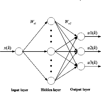
Figure 7. The structure of action network.

Д W ( k ) = l ( k ) ^f - ⁵ E a ^{( k} ) 1

a         A ⁵ W a ₁ ( k ) )

_ l пл f ⁵ Ea ( k ) ⁵ Q ( k ) ⁵ “ ( ^k ) _d V < k L ⁵ ah ²< k ) ⁵ ah1(^k )

= a ( ) ( d Q ( k ) d u ( k ) d v ( k ) d ah 2( k ) d ah1(k ) d W a 1 ( k )

= - ¹ ■ l ( k ) ■ e ( k ) ■ x ( k ) ■ [ 1 - ah 2( k ) ® ah 2( k ) ]

8 aa

® j [ ( W c 2 ^T ( k ) ® (1 - ch 2( k ) ® ch 2( k )) ) X W cu ^T ( k ) ]

x( A(k) ® Wa2 )T} where

W cu = W c 1 (1:3,:)

A ( k ) =[ ( 1 - u ( k ) ® u ( k ) ) ; ■■■ ; ( 1 - u ( k ) ® u ( k ) ) ]

Total 8

It should be noted that, in the formulas above, the operation symbol “ x ” means the general matrix multiply, while the operation symbol “ ® ” means bitwise matrix multiply.

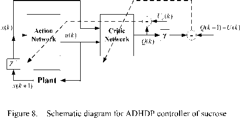
The schematic diagram for ADHDP controller of sucrose crystallization is shown in Fig. 8.

• V.    Simulation Results

The initial Brix of sucrose solution is 83Bx. We choose randomly initial weights of the critic and the action networks in the range of (-1,1). We use l_c ( k ) = 0.3 , l_a ( k ) = 0.3 and / = 0.95 in our simulation. In order to prevent the training of the critic network and the action network from entering the endless loop we set the maximum cycle-index as 50 and 500, respectively. The simulation results are shown in Fig. 9 and Fig. 10..

• VI.    Conclusion

It is quite difficult to establish a precise mechanism model of sucrose crystallization. According to the principle of sugar boiling process, and the practical experience of workers, we developed a neural network model of the crystallization based on the data from the actual sugar boiling process of sugar refinery. The approximate dynamic programming approach can solve the optimization control problem of nonlinear system. The ADHDP as a model independent ADP approach has provided some level of flexibility. The paper covers the basic principle of this learning- and approximation-based approach and the design of neural network controller based on the approach. The result of simulation shows the controller based on action dependent heuristic dynamic programming approach can optimize industrial sucrose crystallization ．

Acknowledgment

The authors would like to thank Dr. Qinglai Wei for his help in preparing this manuscript.

crystallization

Brix of the collation stage

82.5

81.5

81 0

82 0

Time steps

Brix of the enrichmen A and crystallization stags

250   290

100     150     200

Time steps

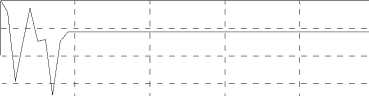
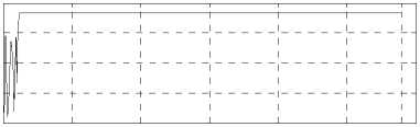
Figure 9. Simulation results for the collation, enrichment A and crystal growth stage.

Brix of the water boiling stage

0       10      20      30      40      50      60

Time steps

Brix of the enrichment B stage

0     5     10    15    20    25    30    35    40

Time steps

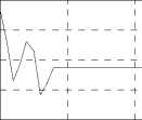
Figure 10. Simulation results for the water boiling and enrichment B stage.