Optimal Playing Position Prediction in Football Matches: A Machine Learning Approach

Published Online on December 8, 2023 by MECS Press

Football is, without a doubt, the most popular sport worldwide. Other popular sports include basketball, tennis, and cricket, but nothing surpasses football's popularity. Globally renowned teams such as Manchester United and tournaments such as the Champions League have insured that football will continue to exist. Football has permeated all aspects of life, as we are continuously assaulted with advertisements and betting offers involving football celebrities. As football is played in numerous nations, it has produced dozens of superstars. Football's popularity rises as a result of the larger number of participants than in any other sport.

With the recent surge of football events in 2022, for example the World Cup, it is evident that football is returning to its former glory as one of the most glorified sports in the world. Incidentally, numerous amateur football players are interested in joining the professional football league. However, as an amateur football player trying to join a professional team on a whim to play professionally isn’t realistic. On the other hand, it is the team manager that handles executive recruitment along with talent identification. Based on [1], talent identification is a very crucial avenue in effort to achieve top class sporting excellence and efficient guidance in any sports.

Usually, talent identification doesn’t happen instantly, potential players would enlist in a practice program that would span from 3-6 months on average. Afterwards, at the end of the program, potential players who boast the most skill and potential will be enrolled in the team, hence enabling these players to play professionally. However, this approach isn’t really recommended for small-medium scaled football teams, this is due to the exorbitant prices on hosting this program. Furthermore, talent searching also requires the skills of experienced analysers who are adequate at their field and discovery of sports talent using Artificial Intelligence (AI) is still incompetent [2]. Likewise, with the incorporation of talent identification, there also lies talent management, which possesses its own sets of importance in football management. In football management, talent identification and talent management go hand in hand. Talent management remains a challenge, especially in ensuring the best position for a player in a team formation. This may be due to the fact that these tasks requires a lot of experience in decision management and coaching. In general, there are no scientific equations or formulas adopted to recognize the most suitable position for each player in a particular team formation [1]. Football manager or team coaches needs to perform many experiments directly with the players and analyse them individually to get an idea of a player’s skills. These featured skills would involve many different aspects such as offensive, defensive capabilities, and supporting capabilities. These areas would affect how the player would blend in into the team and be put in a suitable position [3].Given these various confines, professional sporting organizations are increasingly turning towards machine learning to assist with the identification of players who possess unique attributes in certain playing positions may offer a competitive advantage [4]. To utilize and make talent identification and position selection more accurate for football managers and team coaches, data mining techniques and machine algorithms, primarily classification algorithms could aid in making the correct decisions [3]. These techniques would require data that is accurate, structured, and processed in the first place [5]. For this reason, a model predictor created using various machine learning algorithms are needed and applied to help in giving positions recommendations for football managers and team coaches to players in a football team. The dataset provided for the training of the model predictor will be obtained using web-scraping from a popular football statistics website. Afterwards, the prediction model will then be compared with other common classification algorithms and the algorithm that achieves better results based on its evaluation metrics, using both accuracy and F1-Score, will be selected.

In a previous study done by [4] using Machine Learning approach with the purpose to detect DDoS attacks using various Machine Learning Classification Algorithms has shown exceptional result with most evaluation metrics lying in the 98% mark. Having a high evaluation metrics shows that a model predictor is highly reliable, However the limitation of this study lies in the lack of explanation of how the Machine Learning approach is performed. To be able to understand how an analysis is performed, it should be explained briefly or in detail. Lastly, a past study done by [6] with the same purpose of predicting football player’s position, uses an algorithm called the fuzzy logic, which was applied to 264 soccer players revealed that the system designed using fuzzy logic is able to identify the qualities among players exceptionally well. However, using fuzzy logic in itself requires a good deal of human intervention, primarily needing domain experts who are well-experienced in this area of expertise, therefore relying on another approach, for example Machine Learning using either Supervised Learning and Unsupervised Learning is preferrable because the iterative process is automatic and the machine is able to learn with more training, whereas using fuzzy logic, this process may be cluttered.

2.    Literature Review

Previous have shown various usage of machine learning and classification algorithms, primarily the Decision Tree algorithm in helping individuals and organizations perform prediction. These usages are prioritized and practiced widely in various domains, such as finance, healthcare, marketing, management, and many more. In finance, a study performed by [8] focused in developing a hybrid model called the Hybrid Credit Card Fraud Detection (HCCFD) system using anomaly detection techniques by applying genetic algorithm and multivariate normal distribution to demonstrate the effectiveness in detecting fraudulent credit card transactions. The results of the study showed that the HCCFD system outperformed other used machine learning algorithms such as artificial neural network, decision tree, and support vector machine, with an accuracy of 93.3%, including the Decision Tree algorithm performing relatively well at 79.4%. A separate study carried out by [9] for the cause of predicting football match winner outcomes from the output of the English Premier League using historical match statistic data shows suboptimal results with of the Decision Tree algorithm with an accuracy of 64.87%, hence showing that the model predictor is not suitable in performing the respective tasks. This limitation may be caused by incomplete or faulty data pre-processing. The author also mentioned that the problems were also caused due to overfitting and the trained model had limited data caused from the small size of the dataset with very few features. Therefore, in the study that will be performed these factors will be taken into account.

Moreover, a study by [10] explored various classification algorithms which are KNN, Naive Bayes, Support Vector Machine, Decision Tree, and Random Forest. The use of these algorithms assisted potential bicycle buyers in making informed choices. The classification model developed by the author, using data collected from 242 bicycle users in various communities in Indonesia. The findings suggest that Decision Trees has proven to be useful as a predictive tool for potential bicycle buyers in selecting the appropriate type of bicycle to purchase. Lastly a study by [11] was conducted to analyze the relationship between extracurricular activities and academic performance of students using Machine Learning prediction algorithms such as Decision Tree, Random Forest and KNN. The study focused on discovering the shortcomings in each algorithm and compares the prediction outcomes obtained by these algorithms. Results depicted that the Decision Tree algorithm outperforms other algorithms with an accuracy and F1-Score of 85% and 84% respectively. The author expects that the result of this study will help in paving the way for more specialized and in-depth studies in predicting academic performance of students using machine learning algorithms.

While these studies have demonstrated the effectiveness of Decision Trees in prediction tasks, there are some limitations that need to be considered. For instance, Decision Trees may overfit the training data, leading to poor performance on new, unseen data. To address this issue, researchers have developed various techniques, such as pruning, ensemble methods, and cross-validation, to improve the generalization of Decision Trees. Moreover, Decision Trees may be biased towards certain attributes or features, leading to suboptimal predictions. This issue can be addressed by careful feature selection and preprocessing. In conclusion, Decision Trees have emerged as a powerful tool in the field of machine learning, with various applications in prediction tasks.

3.    Research Methodology 3.1    Block Diagram

The diagram of the Research Process depicts the data science methodology from business comprehension to model evaluation (see Fig. 1). Several parameter tuning procedures were iterated to improve the performance of a machine learning model.

Business Understanding

Data Understanding

Data Preparation

Fig. 1. Diagram of the Research Process

• 3.2    Business Understanding

• a.    Target Variable:

• 1.    Position: Suitable Position for football players

• b.    Features Affecting Target Variable:

• 2.    KeyPasses: Key passes per game of player

• 3.    Dribble: Dribbles per game of player

• 4.    Dispossessed: Dispossessed per game of player

• 5.    BadControl: Bad Control per game of player

• 6.    Playtime: Total playtime of player

• 7.    Tackles: Tackles per game of player

• 8.    Intercepts: Intercepts per game of player

• 9.    Fouls: Fouls per game of player

• 10.    Offsides: Offsides per game of player

• 11.    Clears: Clears per game of player

• 12.    DribblePast: Dribble past per game of player

• 13.    Blocks: Blocks per game of player

• 14.    Goals: Total goals of player

• 15.    Assists: Total assists of player

• 16.    ShotsAveragePerGame: Shots average per game of player

• 17.    PassSuccess: Pass success percentage of player

• 18.    AveragePasses: Passes per game of player

• 19.    Crosses: Crosses per game of player

• 20.    Longballs: Long balls per game of player

• 21.    ThroughBalls: Through balls per game of player

• 3.3 Data Understanding

In this point, analysis of the data will be explained step-by-step to help understand the process in understanding the data used to solve the task which have been explained in the first two points.

• a.    Data Collection

The dataset used for the analysis will be taken and scraped from The steps on how to replicate the process of web scraping will be explained in great detail in this subpoint. To perform web scraping on the consequent website given above, a free extension called Octoparse will be used. Octoparse is a cloudbased web data extraction solution that helps users extract relevant information from various types of websites. To begin, first open up Octoparse. Make sure the newest Octoparse has been installed, currently Octoparse is on its 8th version. If everything has been implemented and installed properly, the main page will be shown (see Fig. 2).

Fig. 2. Main Page of Octoparse

Afterwards, we can then enter in the link of the website that we want to scrap in the search box below the Octoparse logo. Now, after a link has been entered in the search box, Octoparse will redirect us to something called a “workflow” (see Fig. 3), this is the place where we are given the leniency to customize our own web-crawler and webscraper.

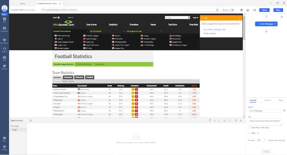
Fig. 3. Workflow of Octoparse

First before we start the crawling and scraping process, we want to analyze the page of the website, there are two main tables present on the website. Firstly, the table for team statistics and secondly the table for player statistics. Based on our task objective, we will take the player statistics table (see Table 1.) instead.

Table 1. Football Player Statistics Table

On top of that, we want to decide the flow or in other words the logic for scraping the specific website. If we examine closely on the table of the player statistics, we can see that there are 5 tabs of which are: Summary, Defensive, Offensive, Passing, and Detailed. Currently we are on the Summary tab, each tab will have its own respective attributes. Hence, these attributes and also the player information from each tab will be scraped. For simplicity purposes the Detailed tab will not be scrapped because it contains real-time statistics and is not suitable for the task we are trying to accomplish. Another thing to note is the pagination present on the table. There are about 145 pages, each with 10 rows of data regarding each individual football player on each page. That being said, the logic for scraping the consequent table would have to take into account these tabs and also pagination routes and options. To make things easier, we will make use of the auto-detect feature on the top right corner of the workflow (see Fig. 4).

Select a page element you'd like to extract from.

Auto-detect webpage data

Check workflow

Fig. 4. Auto-detect Scraping Feature

Subsequently, we then want to click on the auto-detect webpage data link and Octoparse will automatically detect all the scrapable contents on the website (see Fig. 5). Octoparse shows 4 blocks of content that is potentially scrapable. However, since the main focus lies on scraping the player statistics table, we want to focus on this part. Octoparse autodetect feature has already taken into account pagination, so we don’t have to worry about it anymore. In spite of that, there is one caveat regarding this method of web-scraping, which is the inability to switch tabs. It is quite hard to switch tabs and scrape the data due to the structure of the table. Hence, we will create 4 workflows, each with the purpose of getting all the attributes and player information on each tab.

Fig. 5. Auto Detect Result

Following the usage of the auto-detect feature, we then want to click on the create workflow button whilst having the options above checked. Afterwards, we can see that a logic tree/flow tree has been created on the right side of the workflow (see Fig. 6). Indicating the content that we want to scrape and how it will be scrape.

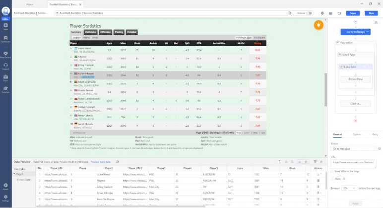
Fig. 6. Flow Tree at the Right Side of the Workflow

Coincidentally, after confirming the flow of the web-scraping process, we then want to proceed on starting the web-scraping process. To do this we can simply just press the run button at the top right corner of the workflow just below the exit program button. Octoparse will then display a modal message whether to run the scraping process via local or cloud, since we are currently using the free version of Octoparse, we will carry on with local devices. After confirming this option, Octoparse will then run the scraping process and scrape all the available content based on the flow tree (see Fig. 7). And after the scraping process is done, Octoparse will send out a notification indicating that the scraping process is finished along with the option to export the data in various different file formats such as xls, csv, etc. For the use of the analysis, we will export the scraped content/data into the csv format.

(® Show Browser)

Football Statistics | Soccer Statistics

О Running

[Loop Item] executing loop item -#7

Duplicates: 0 line(s) Time Spent: 1m 23s Avg. Speed: 36 lines/min

I I Pause          И Stop

Task Overview      Data List Eventlog     Recent Runs # PlayerURL Player                 Playerl                Player_URL2           Player3                Player4                PlayerS                Apps                  Mins 6     https://www, whose,,, 46                     Ivan Toney             https://www,whose,,.   Brentford,              26                    ,. FW                   14                     1260 7     https://www. whose.. 47                     Eric Choupo-Moting Bayern,                33                     , M(CLR),FW           6(4)                    520 8     https://www, whose,,, 48                     Adrien Rabiot          https://www,whose,,.   Juventus,              27                     , DMC,M(L)            11                     935 9     https://www, whose,,, 49                     Leroy Sane             https://www,whose,,.   Bayern,                26                    , M(CLR),FW           8(5)                   840 10 50                     Thomas Partey          Arsenal,                29                    , D(R),M(CR)            11                     961 11    https://www, whose,,, 51                     Randal Kolo Muani     https://www,whose,,.   Eintracht Frankfurt, 24                    , AM(R),FW            13(1)                  1122 12    https://www, whose,,, 52                     Jonas Hofmann        https://www,whose...   Borussia M.GIadba.., 30                    , D(R),M(CLR)          13                     1155 13 53                     Frenkie de Jong         Barcelona,             25                     , D(Q,DMC            9(4)                    898 14    https://www. whose... 54                     Mario Rui               Napoli,                31                     , D(L),M(L)             11(1)                  977 15    https://www, whose,,, 55                     Dominik Szoboszlai    https://www,whose,,.   RBL,                   22                     , AM(CLR)              11(2)                  953 16    https://www, whose,,, 56                     Joelinton              https://www,whose,,.   Newcastle,             26                    , AM(CLR),FW          12(1)                  1060

3   5 Go to Page

Fig. 7. Scraping Data from the Website

We then want to do this for all the remaining tabs, which are the Defensive, Offensive, and Passing Tab. The flow for scraping the content on each respective remaining tab is similar, however the difference lies in adding a simple click listener to navigate between these tabs (see Fig. 8). At first, we start out at the Summary Tab, hence we didn’t need to add a click listener, however the opposite could be said when we are scraping from the other tabs.

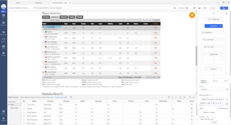
Fig. 8. Added Click Listener to Navigate Between Tabs

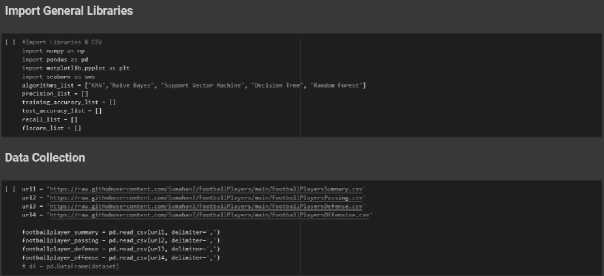
Fig. 9. Importing Csv and Libraries

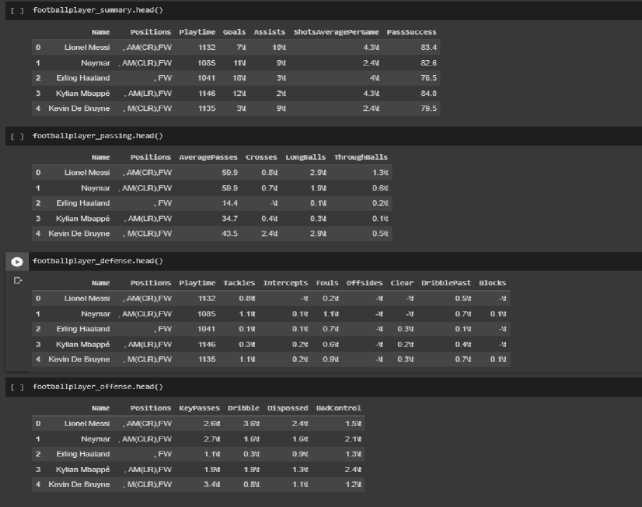
After importing both the csv and libraries, we can then view the overall structure of the dataset using the head() function (see Table 2.). It is imminent that the tables are still relatively dirty and cleaning would need to be operated on each of the tables.

Table 2. View Overall Structure of Dataset Using head() Function

• b.    Data Integration

Table 3. Converting Data into Dataframe and Merging of Dataframes

• c.    Pre-Cleaning

Thereafter the data integration process has eclipsed, a step called pre-cleaning will be performed upon the dataframe. The pre-cleaning step will involve cleaning the table to transform it into something “usable” or able to be processed by the machine learning model. Notice that some of the values on the table ends with “\t” this might have something to do with how pandas read our csv files. But no worries, we can simply replace all values or instances of all features that end with “\t” with a blank string (see Table 4.). Furthermore, we also see that some values are indicated with “-”, the website we scraped data from depicts values that are 0 as “-”, so for the time being we will be replacing all “-” values with NaN to make processing our data much easier in the later points.

Table 4. Replacing Instances that Contains “\t” and “-”

If we were to call the info() function, we can see that most of the features of the data is of type object Z, even though the values contained in all the features are all numerical, except for Position (see Fig. 10). Hence, we need to convert the datatype of the features with the type of object into their own respective data types (int/float).

Fig. 10. Convert Object Features into Numerical

Something else we need to take into account is the position feature. The values of the position feature are still relatively dirty (leading commas, multiple positions of individual football players, whitespaces, and variation of the same values) (see Fig. 11). Based on the task objective we are trying to find the perfect position of a football players we only need one position to do our analysis. Hence, we need to clean and replace the inconsistent values in the position column.

Fig. 11. Position Column Pre-Cleaning

After pre-cleaning the position column. The position column now only contains 6 unique values, which shows the position a football player can be assigned to in a team formation (see Fig. 12).

о df("Position"].unique ()

□- arrayd'AM*, "W, ‘H*, 'O', 'ОМС', '«•], dtype=object)

Fig. 12. All Unique Values of Position Column

• d.    Data Visualization

To get a better understanding of the data we are working with and also gain insight we will be performing Data Visualization, specifically EDA. Exploratory Data Analysis (EDA) refers to the critical process of performing initial investigations on data so as to discover patterns, to spot anomalies, to test hypotheses and to check assumptions with the help of summary statistics and graphical representations [12-14]. We will be dividing the step of EDA Visualization into two categories which are EDA (Univariate) and EDA (Multivariate) [15]. Univariate means the analysis of one variable whereas Multivariate means the analysis of more than one variable.

• e.    EDA (Univariate)

To get a brief layout and structure of the data we can get a sample of the data using the head() function to give us the first 5 instances of the data. Next, we can find the shape of the data using the shape() function which gives us the total number of columns and rows of the data. The data comprises 1460 rows/instances and 21 columns including the target variable. We can divide features of the data into both numerical and categorical. The numerical features are: KeyPasses, Dribble, Dispossessed, BadControl, Playtime, Tackles, Intercepts, Fouls, Offsides, Clears, DribblePast, Blocks, Goals, Assists, ShotsAveragePerGame, PassSuccess, AveragePasses, Crosses, Longballs, and ThroughBalls. The categorical feature of the data is Position. Subsequently, we are then going to research and analyse both numerical features and categorical features of the data.

• f.    EDA (Multivariate Numerical)

Fig. 13. Describe() Function to Get Statistical Description of Data

We can further enrich our knowledge and information about the numerical features of the data using the describe() function, which gives a lot of statistical information of the data (mean, range, std, etc) (see Fig. 13). A good insight to be drawn from these visualizations is regarding the range of the data: the range of the data of all the features lies between 0.1 until 1350. The difference between the ranges of these data may be major but we will normalize these values during the data pre-processing step. Another thing to note is that the count of the data is not the same for each of the features, this is because during the pre-cleaning step, we transformed all “-” values into NaN to make it easier for us to process the data later on.

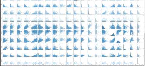
Fig. 14. Pair Plot between the Numerical Features of the Data

We can use a pair plot to analyse numerical features with respect to other numerical features (see Fig. 14). A good thing to note in this analysis is regarding the line of best fit. Hence, we can draw a line of best fit with respect to other numerical features, therefore we can categorize this visualization of the graph as linear (if one of the features is high, then the target variable is also high). We can detect a crucial thing regarding the graph, which are “outliers”; the outliers are present on the left side of the graph and may have a considerable impact on the prediction of the data.

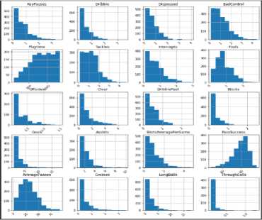
Fig. 15. Histogram of All Numerical Features

Next, we can see the data distribution of each feature using a histogram (see Fig. 15). From the histogram, we can conclude that most numerical features are skewed to the right. With the exception of PassSuccess and Playtime. Generally, if data distribution is skewed to the right then that means that potential outliers of the distribution curve are further out towards the left. And the opposite could be said if the data were to be skewed to the left.

• g.    EDA (Multivariate Categorical)

Similarly, with the EDA of the numerical features, we can use describe(include=”object”), to get statistical information of the categorical features of the data (unique values, frequency, etc) (see Fig. 16).

' Categorical Feature

Q ttf.describe(irKlude='object'} position ^-count1460

unique6

freq548

Fig. 16. Categorical Feature Statistical Description

Afterwards, we can then view the distribution of unique values of the categorical features using a bar graph (see Fig. 17). The insights we got from the bar graph is that most of the football players of the dataset have a position of a Defender whilst Goalkeeper having the least. We can also then use a pie chart to illustrate the numerical proportion of data in percentages (see Fig. 18).

Fig. 17. Position Distribution using Bar Graph

Fig. 18. Position Distribution Percentages using Pie Chart

• h.    Data Preparation

In this point, pre-processing of data will be explained in detail. Pre-processing of the data is done to prepare (cleaning and organizing) the data to make it suitable for building and training the Machine Learning model [16]. Afterwards, the determining and dividing of data into dependent and independent variables, along with splitting the data into training and testing will be performed. Lastly, oversampling will be applied due to imbalance data across the values of the features and feature scaling will be applied on the independent variables to make the process more accurate.

• i.    Filling NaN Values

As touched upon the earlier parts of the analysis, specifically on the Data Understanding phase. We have converted all “-” values into NaN, therefore we will fill these null values with 0 (see Fig. 19).

Fig. 19. Filling NaN Values with 0

• j.    Deciding Dependent and Independent Variables

The next step of data pre-processing is splitting our features into dependent variables and independent variables. The target variable (y) is the Position of the player because we want to classify football players into the perfect position based on team formation, underpriced or standard priced based on the dependent variables. Hence the other variables affecting the target variable will be the dependent variables (X). Since we are trying to make a classification model to predict a player’s position based on these dependent variables.

• k.    Balancing Imbalanced Data

Subsequently, we want to then balance the classes in our target variable. Balancing imbalance data is important because it makes training a Machine Learning model easier as it prevents the model from being biased towards one class just because it contains more data [17]. The balancing method that will be used is Random Oversampling. If we see the classes of the Position Column, we can see that Defender has 548 instances and Goalkeeper has 92 instances. Hence, balancing of these classes are needed due to the reason above. To do this, we will be using Random Oversampling. As the name suggests, this is a technique that randomly selects points from the minority class and duplicates them to increase the number of data points in the minority class. Oversampling is the most suited instead of under sampling because, if we were to delete part of the majority class then the accuracy of training the model will be reduced and clarity will be lost [17]. Subsequently, the sample might not accurately represent the real world and may cause the analysis to be inaccurate.

• l.    Feature Scaling

After balancing our target variable value, we then want to do feature scaling on our variables. Feature scaling is one of the most important data pre-processing steps in Machine Learning. Algorithms that compute distances between features tend to have numerically large values if the data is not scaled [18]. Hence, we will be applying a feature scaling technique called Standardization (see Fig. 20). This is made possible using a sklearn library called StandardScaler. The reason why we would want to standardize our data is because our data comes in varying ranges and has a normal distribution. By standardizing our data, we do not have to take in account data distribution anymore. Hence, using standardization we are able to transform every feature of our data so they have the same dimension to remove redundancy and repetitiveness [19]. Furthermore, standardization is not affected by outliers, because there is no predefined range of transformed features.

Fig. 20. Feature Scaling with Standardization

• m.    Train and Test Split

After standardizing the data, we want to split our data into training and testing data. We split our training data and testing data with a ratio of 0.7 and 0.3 respectively.

• n.    Modeling

In this point the process of creating a machine learning model will be elaborated. Five classification algorithms will be used to create our Machine Learning model. The classification algorithms used are: KNN, Naive Bayes, Support Vector Machine, Decision Tree, and Random Forest. Afterwards during the Evaluation step, the best model based on the classification algorithms used will be chosen and explained.

• o.    Maximizing Parameter

Before we create a model, it is advisable to first find the best parameter to maximize the performance of the Machine Learning model. To achieve this, a sklearn library called GridSearch will be used. A good thing to note is that each classification algorithm has their own set of parameters and differs from each other. Therefore, when we use GridSearch, we won’t be maximizing the same parameters over and over.

• a)    Parameters to be maximized in the KNN Algorithm as recommended by [20] (see Fig. 21) :

• • n_neighbors: Number of neighbors defined

Fig. 21. Finding Best Parameters for KNN Algorithm

• b)    Parameters to be maximized in the Naive Bayes Algorithm as recommended by [21] (see Fig. 22):

• •    var_smoothing: The portion of the largest variance across all features

  

petnt(re№oeijr3d.pest_«ttewj orinKiWOdeljid.bestjureJ

Fitting s folds for e«h of iee candidates, totalling see fits

Gnjssiaiwp(v3r »ootntiv^a.iMMnei»?B606iitir. >

{■«■"..senthuio': e.ee23iei:s?eeesii6e5i

Fig. 22. Finding Best Parameters for Naïve Bayes Algorithm

c) Parameters to be maximized in the Support Vector Machine Algorithm as recommended by [23] (see Fig. 27):

• •    kernel: Kernel type to be used in the algorithm

• •    C: Strength of regularization

• •    gamma: Kernel coefficients

Fig. 23. Finding Best Parameters for Support Vector Machine Algorithm

d) Parameters to be maximized in the Decision Tree Algorithm as recommended by [23] (see Fig. 24):

• •    criterion: The function to measure the quality of a split

• •    max_depth: Maximum depth of tree

• •    min_samples_split: Minimum number of samples to split an internal node

• •    min_samples_leaf: Minimum number of samples required to be at a leaf node

Fig. 24. Finding Best Parameters for Decision Tree Algorithm

e) Parameters to be maximized in the Random Forest Algorithm as recommended by [24] (see Fig. 25):

• max_features: The number of features when looking for the best split

• max_depth: Maximum depth of tree

• min_samples_split: Minimum number of samples to split an internal node

• min_samples_leaf: Minimum number of samples required to be at a leaf node

Fig. 25. Finding Best Parameters for Random Forest Algorithm p. Creating and Training Model

After having found the best parameters for each algorithm, we then want to create our model. Hence, why we used GridSearch to find the best parameter when we want to create our Machine Learning model. To create a model, we need to use the respective algorithms classifier from sklearn (see Fig. 26). Afterwards, we can then train our model so that our model will learn how to understand and deal with unknown data when we test our model, to predict the best position for a football player (independent variable) based on the features (dependent variables) [25]. Or in other words we train our model so that it can learn patterns in the data.

Fig. 26. Creating Various Models Using Best Parameters from GridSearch

3.    Evaluation

In this point the metric evaluation of the model will be provided, the explanation for choosing the metrics, and choosing as well as explanation of the best model based on the evaluation metrics. Evaluation acts as the final step of Machine Learning. The reason as to why that is the case is because, if we have a Machine Learning model and have trained it beforehand. How are we going to test whether our model has successfully solved the problem at stake? How do we know whether our model did find a solution to the problem and how efficiently did they do it? These are some of the questions asked during the evaluation step. If all these questions are able to be answered correctly, then we can say that our model is marked as worthy and reliable.

• A.    Reasons of Using Specific Evaluation Metric

The evaluation metrics used for the specific analysis will be related to the type of task that is used. Because we are creating a Machine Learning model to do classification, therefore we will be using evaluation metrics that are suitable to evaluate a classification model. Every evaluation metric in a classification model will be based on the confusion matrix. Confusion matrix is essentially a performance measurement/indicator that provides details in the form of true/false labels which classes are being predicted correctly, incorrectly, and the errors that may have been made by the model [26]. There are four outcomes in a confusion matrix. First case is where a prediction is said to be true and it comes out as true (True Positive), second case is where a prediction is said to true and it comes out as false (False Negative), third case is where a prediction is said to be false and it comes out as true (False Positive), and lastly the case where a prediction is said to be false and it comes out as false (True Negative) [26]. After receiving and determining a confusion matrix can we then use the other evaluation metrics of a classification task. Hence, the evaluation metrics used in these analyses will be: Accuracy, Precision, Recall, and F1-Score. Accuracy is an evaluation metric in the classification task that looks at the True Positives and True Negatives of the confusion matrix and measures how many times a model got the prediction right [27, 28]. The reason as to why Accuracy is used as one of the evaluation metrics is because Accuracy is a very popular evaluation metric in classification and it is very easy to interpret for people who may not have a Machine Learning background. Another reason is because of the nature of our task analysis, since we are trying to predict the perfect position for a football player in a team formation, it is necessary for the model to be able to predict correctly most of the time, so it can maximize a team’s performance by assigning talented football players in their ideal position. Precision is another evaluation metric that is used, which focuses on how precise the model is in predicting positive labels, therefore True Positives and False Positive outcomes from the confusion matrix will be used [27, 28]. Precision is helpful in calculating how many times when a model predicts as positive and counted as correct. This is especially a very crucial thing to take into consideration, if the model were to predict in the case of a Forward Winger, for example, the football player's best position to be a Defender, whereas in reality he is a very good Forward Winger. This is proven to be detrimental in managing a football team's quality and performance. These two positions are very different from each other, where Defenders mostly have a very defensive playstyle and usually play in the backline, stopping opponents from reaching the goal. Whereas Forward Winger plays upfront trying to look for every opportunity to make key passes to their teammates and score assists and even goals. The next evaluation metric that will be used is Recall. Recall is the calculation of percentages of actual positive the model identified as correct [27, 28]. Recall is very useful as an evaluation metric, let’s say out of 10 predictions in the case of Defender. The model was able to correctly identify all the players as Defender, hence it will maximize a team performance with this regard because more roles are being filled in a football team and the team’s quality is maximized. Lastly, the evaluation metric used is F1-Score. F1-Score is regarded as one of the most important evaluation metrics in a classification task. F1-Score is the harmonic mean of precision and recall and therefore is considered as the sum of predictive performance of the model based on precision and recall values [27, 28]. In other words, it combines both precision and recall values into a single number. F1-Score also takes into account both False Positives and False Negatives, meaning that if Recall and Precision score are high that means F1-Score is also high. The closer the F1-Score is to one then the model is considered good/reliable.

• B.    Cross-Validation

To make the most out of the evaluation metrics, a method called Cross validation will be performed on the model. Cross validation is a step that is performed right after we train our dataset. If we were to do just testing after training our model, it may not be real-world worthy, because it only represents a small set of all the possible data. Since the main objective, is that the model we have trained should be adaptable to the real-world and applied without any faults. Cross validation will be used to estimate the performance of a Machine Learning model based on the previously defined evaluation metrics and is especially useful in protecting our model from overfitting [29], [30]. In cross validation, we make a fixed number of folds (or partitions) of the data, run the analysis on each fold, and then get the average of the evaluation metric [29], 30]. The cross validation that will be performed on the data will have a fixed number of 10 folds. Hence, we will perform cross validation on all the classification models (KNN, Naive Bayes, etc) and get the average score of the evaluation metrics after running the partition 10 times (see Fig. 27).

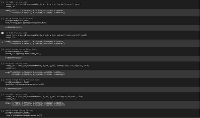
Fig. 27. Performing Cross Validation of the Evaluation-Metrics

• C.    Summary of All Models Evaluation Metrics and Choosing of Best Model

Based on the evaluation metrics that have been obtained from the Cross Validation step (see Table 5.), we can see that the Naive Bayes model has the lowest score of all evaluation metrics. Therefore, we are crossing off Naive Bayes from the selection of the best model. Following up is the Support Vector Machine model. Although the model may have high evaluation metrics, it is overfitting the model by approximately 9% based on the difference of the testing and training accuracy. The difference of 9% here is a big deal, because even if all Machine Learning models overfit, we want to minimize overfitting to a small margin whilst also having a reliable evaluation of the model. As a consensus, we are crossing the Support Vector Machine model for the candidate of best model. Similarly, due to the high value of difference, which causes overfitting in copious amounts, we are also crossing off KNN from the selection. Now we are just left with both Decision Tree and Random Forest. These two models are very similar, due to the fact that the Random Forest model is just a collection of decision trees. However, we will not be focusing on how similar a model is to each other, comparison will only be done based on the evaluation of the models. From both of the models, we can see that they experience overfitting on the range of 1.4% to 2.0% respectively based on the training accuracy and testing accuracy difference. The difference between these values is minimal, this is why we must also take into account the evaluation metrics of both the models. For example, the evaluation score of the Random Forest model is inferior to the evaluation score of the Decision Tree model. Taking this into account, we will pick the Decision Tree model as the best model used to classify the perfect position of football players based on a team formation. Hence, the evaluation score of the Decision Tree model is as follows:

• 1.    Testing Accuracy: 0.760998

• 2.    Precision Weighted: 0.769015

• 3.    Recall Weighted: 0.767089

• 4.    F1-Score: 0.753640

5.    Conclusion

Table 5. Result of the Evaluation Metrics of Each Algorithms

	Algorithms	Training Accuracy	Testing Accuracy	Precision	Recall	Fl-Score
0	K1JN	0 774882	0718367	0.721657	0.718367	0714414
1	Naive Bayes	0.688869	0.690961	0.694605	0.690961	0.679167
2	Support Vectoi Machine	0.896569	0.804504	0.805040	0.804504	0.800687
3	Decision Tree	0.780975	0.760998	0.769015	0.767089	0.753640
4	Random Forest	0.717090	0.703257	0.706274	0.705164	0.685706

The study that has been conducted utilizes various machine learning algorithms of which are k-nearest neighbor, naïve bayes, decision tree, support vector machine, and random forest. Creation of the model predictor, data collection, data analysis, and data processing were accomplished using the Python programming language, machine learning library (sklearn), and Octoparse for the purpose of data collection through web crawling and web scraping.

As a conclusion, the model predictor that has been designed proves to be competent enough to the extent that it is able to predict and find best playing positions of football players. By using multiple classification algorithms, we were able to conduct trial and error, by finding the best model out of the various models that have been used. This result of this study created using machine learning will prove to be useful in helping football managers, team coaches, and individual football players to discover most suitable playing positions of football based on various attributes that has been defined. Although various confines exists as it has been proven difficult to reach extravagant evaluation metrics or rather exceptional performance due to the fact that in the real world, this result can also be affected by personal decision of individual football players or football managers. Regardless of this fact, we can draw various conclusions from the result of the analysis that has been conducted:

• 1.    The implementation of machine learning can be done to predict and find football player’s playing positions with an accuracy and f1-score of 76% and 75% respectively..

• 2.    The classification Algorithm most suitable to create the model predictors is by using the Decision Tree Algorithm with the highest accuracy, precision, recall, and F1-Score after having taken into account overfitting and underfitting.

• 3.    Algorithms that are not recommended for creating the model predictor are K-Nearest Neighbor and Naive Bayes.

• 4.    High values of overfitting are eminent in both the KNN and Support Vector Machine algorithms.

• 5.    In this analysis, data balancing was proven effective because the number of data copied from the minority class by using the oversampling technique was not done repetitively in large numbers.

• 6.    Proving the best implementation of machine learning algorithms and implementation of data processing can only be carried out by trial and error, this is due to the varied characteristics of the data.

As for future improvements, data sets should be prepared with more features and advanced data cleaning should be performed to maximize the performance of the model predictor in finding the best playing positions for football players. Another improvement would be to use data set that is move varied due to the fact that the data used was obtained using web-scraping from only one source, therefore multiple sources should be used to have more variation in the data to mimic real life scenarios better, hence being able to be formally applied in the football industry in the future.