Optimal Solution to the Capacitated Vehicle Routing Problem with Moving Shipment at the Cross-docking Terminal

Optimum design of a supply chain (SC) is extremely important in the growth of any business in order to stay in a highly competitive global market. In SC system, suppliers/manufacturers, distribution centers and customers/retailers are the key elements. Receiving, sorting, storing, order picking and shipping are the main functions of warehousing in traditional distribution centers. More than 30% of the total production cost is due to the operations at the distribution centers [1]. Some products such as fast moving items with constant demand, perishable items that need immediate shipment and high quality products that do not need quality inspections during the receiving process could be delivered without delay.

To make SC smooth and optimum, an innovative and creative docking technique known as Cross- docking (CD) strategy was initiated in 1930s. However, it only became popular from 1980s after the successful experience of Walmart [1]. CD is a special type of warehousing, where the products which are received are loaded immediately within 24 hours through the shipping door. Since the substantial cost of warehousing is the storage and handling, CD has the ability to reduce the distribution cost significantly. Since space for storage and cost for order picking is significantly small in CD strategy [2], up to 70% of the cost of warehousing can be reduced by implementing CD strategy in SC. The CD strategy in SC can be mostly applicable to the sectors such as pharmaceutical industries, vegetable and flower markets, frozen food and dairy products including beverages distributing companies, courier service providers and e-commerce organizations. Three levels of decisions are involved at the Cross-docking terminal (CDT) and they are strategic, tactical and operational. Strategic level consists of networking the CDT whereas layout of CDT is considered in the tactical level. However, this study is concerned only on operational level and it has several problems to be solved. Vehicle routing between suppliers to CDT and CDT to customers is one of them.

Vehicle routing problem (VRP) is one of the key combinatorial optimization problems in the operations research and is a generalization of travelling salesman problem. It makes an essential part of SC and plays a significant role to make SC smooth and optimum. VRP was proposed by Dantzig and Ramser in 1959 [3]. It has several variants, but this study is only concerned on capacitated vehicle routing problem (CVRP). The research on VRP with CD (VRPCD) was initially conducted in 2006 [4]. Since then VRPCD has gained a lot of attention among researchers and as well as practitioners. Past studies revealed that, the research on transportation problem compiled with CD has been greatly increased. More than 85% of the reviewed research papers on CD were published after 2004 [5]. It is recommended in the literature reviewed [6] to put restriction on scarce resources which are used at CDT by introducing relevant constraints to the model to address for more realistic situations. Further it directs that to focus on internal operations between indoors and outdoors of a CDT. This study attempts to overcome the limitations of considering internal operations in the development of VRPCD model. The unloading products from inbound vehicles, moving unloaded products from indoors of CDT to outdoors of CDT and reloading products to outbound vehicles are some of the internal operations taken place inside a CDT. In this study, these internal operations are also taken into account when developing VRPCD model.

Since 2006, researchers had done several studies on VRPCD by applying different solution methods to the previously published model presented by other researchers. In some past studies, the additional characteristics of VRP were incorporated to the previously published models by others. However, the internal operations are not considered in those studies. In this study, the similar model presented by [4] is considered by relaxing the assumption of simultaneous arrival of inbound vehicles and some internal operations at CDT are added newly. This study differs from the literature in three aspects. Firstly, since almost all the studies find in the literature do not consider the activities inside the CDT and as per the recommendation of [6] to focus on internal operations between indoors and outdoors of a CDT, in this study moving shipment from indoors after unloading the products from inbound vehicle to outdoors, to upload them to outbound vehicles is taken into consideration. Secondly, simultaneous starting time to load the products to outbound vehicles is considered. Thirdly, loading and unloading shipment at all the nodes including CDT is also taken into account. Therefore, the objective of this study is to minimize the total cost which includes not only the transportation cost between nodes but also the cost of moving shipment inside the CDT, vehicle operation cost and service cost at the nodes and as well as at CDT while considering the above mentioned three aspects in addition to the usual VRPCD constraints.

The rest of this study is organized as follows: Section 2 represents the literature review. Problem under investigation in this research is described in Section 3. Section 4 exhibits the mixed integer non-linear programming model associated with the problem under investigation. Computation experiments of randomly generated data are reported in Section 5. Concluding remarks based on the outcome of the study and the recommendations for future research are discussed in Section 6.

2.    Previous Studies

The objective of the primary research [4] on integrated VRP and CD was to determine the optimal vehicle routing schedule and number of vehicles in VRPCD such that to minimize the cost of transportation and the fixed cost of vehicles used in the process by employing Tabu search (TS) algorithm. Two sets of homogeneous fleets of vehicles were used in both pickup and delivery processes. Further, in considered model, it was assumed that the vehicles at the pickup process must arrive CD simultaneously. Hereafter, in this study, for convenience, the model developed by [4] is referred as “Model 1”. Subsequently, [7] applied a modified Tabu search algorithm to solve Model 1 and obtained relatively better solution with less computational time. In addition to the assumptions made in Model 1, multi commodity, heterogeneous and splitting pickup and deliveries were taken into account in [8]. It showed the capability of its proposed model using small-scale problems by solving them using GAMS software. Later, a hybrid method incorporating the elements from the metaheuristics Particle Swam Optimization (PSO), Simulated Annealing (SA) and Variable Neighborhood Search (VNS) were applied in [9] to solve the Model 1 and its computational results revealed that the hybrid metaheuristic yielded significantly better solution than TS algorithm presented by [4]. Heterogeneous property was considered with Model 1 in the studies [10,11] .

Adaptive memory Artificial Bee Colony (ABC) algorithm used in [10] outperformed [7] and the results of SA used by [11] indicated that this algorithm was applicable and effective in solving Model 1 with heterogeneous fleet of vehicles. The open VRPCD for Model 1 was introduced by [12] and to solve the model, SA algorithm was employed. Results for large-scale instances outperformed results obtained from the CPLEX solver not only in accuracy of the solution, but also the computational time to reach the solution. Another SA algorithm was proposed in [13] and obtained better solution for most of the instances in [7]. A metaheuristic algorithm, which decomposed into two phases as Adaptive Large Neighborhood Search (ALNS) and Set Partitioning Problem (SPP), was proposed to solve Model 1 in [14]. That metaheuristic method outperformed the state-of-the-art algorithms in terms of solution and computational time. In [15], better solutions were obtained with benchmark instances using ALNS algorithm for Model 1. Multi commodity property was added to Model 1 in [16] and used CPLEX solver. Optimal solutions for the Model 1 were obtained for 10-nodes instances. However, it consumes a higher computational time for 30-nodes instances. Therefore, heuristic approach was recommended to solve medium and large scale instances by [16].

An extension of the primary study [4], a more generalized and realistic problem was proposed in [17] by relaxing the condition that simultaneous arrivals of pickup vehicles. Instead, the authors introduced dependency rules and consolidation decisions. Also, they considered the corresponding relationships between suppliers and customers. Rather than the different sets of vehicles for pickup and delivery processes used in the previous studies, the same fleet of vehicles was used for both processes. In addition, the time window (TW) in VRPCD was introduced in it. Throughout our study, this model of VRPCD is referred as “Model 2”. A multi-source VRPCD of Model 2 was dealt in [18]. It concluded that, the effect of different consolidation decisions seems to be relatively smaller and cost may increase if different fleets of vehicles used in both processes. A constructive heuristic algorithm to solve Model 2 was proposed in [19] which is different from previously proposed algorithms and it can be found better solutions for most of the instances in the literature. Also, it recommends that this method is suitable for last minute planning as it needs less computational time. The splitting delivery was allowed in [20] and a hybrid algorithm coupled with Ant Colony System (ACS) and SA, was applied to solve the Model 2. The results showed that this hybrid algorithm performed better than applying SA alone.

A metaheuristic algorithm based on LNS was introduced in [21] to solve Model 2. This method enhanced many of the previously best known results. A modified VNS hybridized with GA for the Model 2 was applied to maximize the total profit of the cross-docking system in [22]. It was concluded from its computational results that the proposed hybrid algorithm is more efficient than using the VNS and GA algorithms separately. A new generalized VRPCD was introduced in [23] by extending the dependency rule to many-to-many correspondence between suppliers and customers. Also, in its model, different sets of heterogeneous fleets of vehicles with splitting orders characteristics were considered. Its adaptive memory programming with Tabu search provided similar solutions to [17] and more promising solutions than the solutions obtained in [19]. Branch and Price (BP) algorithm was introduced in [24] to solve small-scale instances of Model 2. It concluded that, BP clearly dominates Linear Programming based Branch and Bound (LPBB) method. To avoid the symmetrical solutions in [24], a novel exact algorithm to solve Model 2 was presented in [25] by introducing a newer Column Generation (CG) technique. Another BP method to solve VRPCD with TW was tried out in [26] to solve moderate-size instances of Model 2. In [27] simultaneous arrivals of pickup process and soft TW were added to Model 2. Its computational experiments indicated that the proposed TS algorithm performed better than VNS algorithm. A mixture of open-close VRPCD with splitting was attempted in [28] and the computational results of two different strategies in SA algorithm were compared.

3.    Problem Description

This study is an extension of VRPCD formulated in Model 1 and referred to it as vehicle routing problem with moving shipment at the crock dock (VRPCD-MS). A typical network of VRPCD is presented in the Fig.1 to illustrate the general structure of the pickup and the delivery processes integrated with CD:

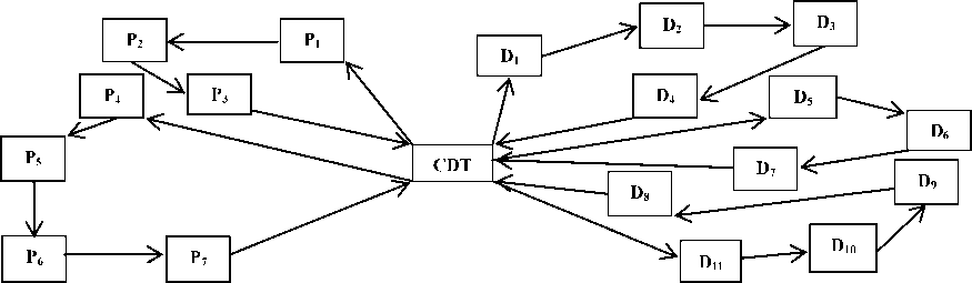
Fig. 1. A network of VRPCD

In this VRPCD-MS problem, all the vehicles start their routes from CDT. The orders of customers are collected from the single product suppliers by fleet of homogeneous vehicles. The collected products are shifted to CDT to unload them at the indoors of CDT. Subsequently, those unloaded products are moved near the outdoors of CDT for consolidation process. Afterwards, they are loaded simultaneously to outbound vehicles (homogeneous vehicles but with different capacity from inbound vehicles). The loaded products are delivered to relevant customers. Finally, all the outbound vehicles return to CDT at the end of their routes. Fig.2 represents the entire process of this transportation problem and followed by the step-by-step procedure to explain all three processes in a SC in detail:

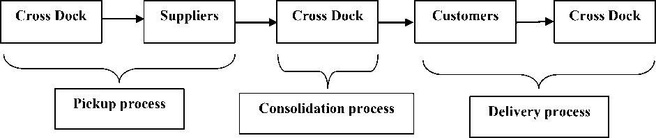
Fig. 2. Integrated processes of VRPCD

• 3.1    Pickup process

Step1 : According to the requests of all the customers, the orders are placed at the suppliers.

Step 2 : The randomly selected node (node i ) is assigned to a vehicle (vehicle k ) which should start its route from CDT.

Once node i is reached, A units of preparation time and B units of time per pallet to load the products have to be considered in order to calculate the service time spent at each node [for example, service time at node i = A + Bt x qt

where q is the quantity to be collected at node i ].

Step 3 : From node i , another randomly selected node (node j ) is assigned to the same vehicle k provided that vehicle k does not exceed its capacity.

Step 4 : If the capacity of vehicle k exceeds, the node j to be assigned to a new vehicle (vehicle l ) which also should start its route from CDT.

Step 5 : Continue Step 3 and Step 4 until all the suppliers are assigned to any of the inbound vehicles used at the pickup process.

• 3.2    Consolidation process

Arrival time of each inbound vehicle from the pickup process is calculated when it reaches the receiving doors of CDT after collecting products in its particular route.

Step 6: After reaching the receiving doors, A units of preparation time and B units of time per pallet to unload the collected products from pickup process in a particular route are applicable unloading time at receiving doors of CDT = A + Bt x

Z q i

Step 7 : Unloaded products at CDT are moved from receiving doors to temporary storage area located at CDT closer to shipping doors. Here, B units of time per pallet is applicable to calculate the time to start the loading at shipping doors in CDT.

moving time from receiving doors to shipping doors at CDT =

B t x Z q i

The outbound vehicle cannot start reloading until all the products are moved to the temporary storage area from the receiving doors. Therefore, the ready time at the shipping doors is the time at which orders are ready to be reloaded in their corresponding outbound vehicles.

Step 8 : Demands of customers are consolidated according to their requests. Also in this case, loading times at shipping doors of CDT (similar to Step 6 ) are determined.

• 3.3    Delivery process

• 3.4    Components of total cost

Step 9 : Step 2 to Step 5 are followed during the delivery process as well.

Step 10 : After completing the delivery at the last node in that route, the outbound vehicle should return to CDT.

It is emphasized that the entire process should be completed within 16 hours.

In this subsection, the components of the total cost to be minimized are categorized as follows:

Transportation cost : Cost of travel in between nodes including CDT. It is assumed in this study that these costs are symmetric; cost of travel from node i to node j is equal to the cost of travel from node j to node i .

Service cost at nodes : The cost for loading products at the pickup nodes and cost for unloading products at the delivery nodes.

Service cost at CDT: The cost for unloading accumulated products by a vehicle (collected through a particular pickup route) at the indoors of CDT and cost for loading products by a vehicle (to be distributed in a particular delivery route) at the outdoors of CDT.

Moving Shipments cost : The cost of moving the unloaded products from each inbound vehicle at the indoors of CDT to load them to the outbound vehicles at outdoors of CDT (or to the temporary storage area at CDT).

Vehicle operational cost : The cost for the maintenance of the vehicles of CDT or the hiring cost of vehicles from the third party.

It is noted that, service cost at CDT and shipping movement cost inside CDT are considered as the cost due to the internal operations at CDT.

4.    Proposed Technique 4.1    Indices i ,j ,h : Indices for nodes (suppliers, customers and receiving / shipping doors of CDT respectively)

k : Index for vehicles

• 4.2    Sets

  N = { P i , P p ,...,	P n , D 1 , D 2 ,..	., D n ‘ }	:     Set of nodes [pickup ( P ) and delivery ( D ) nodes]
  P = { P , P 2 ,...,	Pn }		:     Set of n pickup nodes (suppliers)
  D = { Dx, D p ,..	, D n ‘ }		:     Set of n' delivery nodes (customers)
  V p = { v , v p ,..	., v m }		:     Set of m inbound vehicles
  V d = { v d , v d ,..	, vm, ‘ }		:     Set of m' outbound vehicles
  V = { v p , v p ,...	, vm p , v 1 d , v 2 d , .	.., vm, ‘ }	:     Set of vehicles (inbound and outbound vehicles)
  O = { o , o ' }			:     Set of receiving ( 0 ) and shipping ( 0 ) doors of CDT
  4.3 Parameters

tt :     Travelling time from node i to node j tc :    Transportation cost from node i to node j q :     Quantity (supply/ demand) at node i

Q_p :    Maximum capacity of inbound vehicles

Q :    Maximum capacity of outbound vehicles m :    Number of used inbound vehicles m':    Number of used outbound vehicles ock :   Operational cost of vehicle k (inbound ocpk and outbound ocdk )

st k :   Service time at node i by vehicle k sck :   Service cost at node i by vehicle k dt k :  Departure time of vehicle k at node i at k :  Arrival time of vehicle k at node i

RT_O< :  Ready time at shipping doors of CDT to load the quantity to outbound vehicles

A :     Fixed time of preparation for loading/ unloading products at nodes

B :     Variable time of loading/ unloading a pallet of the product at nodes

A :     Fixed cost of preparation for loading/ unloading products at nodes

B :     Variable cost of loading/ unloading a pallet of the product at nodes

T :     Total time of the entire process

4.4 Variables

k xij

1 , if vehicle k travels from node i to node j 0 , otherwise

• 4.5    Objective function

Minimizing Total Cost (TC) = transportation cost between pickup nodes and delivery nodes + service cost at each node + service cost at CDT + shipping cost from receiving doors to shipping doors of CDT + vehicle operational cost:

MinTC =

(_        ^

z z tcx _v k e V i , j e N и O       7

+

z z sc;x$ kEVieN и O

(    j e N

W     7

+

zz schxk kEVieN HeO

+

z z qA keV ieP j EP и{ О }

+ zz x k e V j e N ( H e O

• 4.6    Routing constraints

All vehicles leave from CDT to pickup or delivery nodes z xkj < 1 V k e V , Vh e O(5)

j E N

All vehicles arrive at CDT from pickup or delivery nodes zxk < 1 V k e V , Vh e O(6)

i e N

One vehicle has to arrive at one pickup or one delivery node zz xk = 1 V j E N(7)

i E N и Ok e V

One vehicle has to leave at one pickup or one delivery node zz xk = 1 V i E N(8)

j E N и O k e V

Preventing loops in routes xk = 0  V i E N и O, Vk E V(9)

Preventing backward movement routes xik + xk < 1 V i, j E N и O , Vk E V(10)

• 4.7    Capacity constraints

Equilibrium condition (Total demand must be equal to total supply) z qi =z qi(11)

iEPi

Vehicle capacity of inbound vehicles z qixk < Qp    V k E Vp(12)

i e P jE P и{ О }

Vehicle capacity of outbound vehicles

£  qiXk < Qd    Vk e Vd(13)

i e D j eD и{ о'}

Number of used inbound vehicles leave from CDT m = ££ ^j(14)

k e V p j e P

Number of used outbound vehicles leave from CDT m ‘=££ tj(15)

k e V_d j e D

• 4.8    Time constraints

Service time at pickup or delivery node

STj = At + BtqjXy    V i e N и O, V j e N, V k e V(16)

Service time at CD (unloading/ loading from inbound/to outbound vehicles)

ST = A t + B t £ q i X ij    Vk e V , V h e O

i e N j e N и O

Departure time of a vehicle k from node i to node j

DT j = ( DT i^k + tt ij + ST j ) x ^k

V i e N и O , V j e N , V k e V

Arrival time of vehicle k at node j starting from node i

AT j = ( tt ij + DT ik ) x ij

V i e N и O , V j e N , V k e V

Ready time at shipping doors of CDT for loading quantity to outbound vehicles

RT , = max <  k e V

ATo + STo + £ qiXik- i e P jeP u{ o }

Departure time of outbound vehicle k from CDT

DT ok = RT_o ‘ + ST j ,    Vk e V

Time planning horizon

max { ATj } <  T k e V

Binary integer values of the decision variables

x k = {0,1} V i , j e N и O , V k e V

• 4.9    Calculation of components of costs

• 4.10    Solution Approach

Service cost at pickup or delivery node

SC ^k _j = A_c + B_cq_jx_i ^k _j ∀ i ∈ N ∪ O , ∀ j ∈ N , ∀ k ∈ V                        (24)

Service cost at CDT (unloading/loading from inbound/to outbound vehicles)

SC_h ^k = A_c + B_c ∑ q_i x_i ^k _j ∀ k ∈ V , ∀ h ∈ O                          (25)

i ∈ N j ∈ N ∪ O

Table 1. Parameter values

Parameter	Value	Parameter	Value
tt ij	Uniform (20, 100)	ocd k	100
tc ij	Uniform (50, 200)	At	10
qi	Uniform (10, 50)	Bt	1
Q p	80	Ac	10
Qd	50	Bc	1
k ocp	150	T	960

5.    Experimental Results 5.1    Results of small-scale instances

It was observed from Table 2 that, in almost all the problems, when it executes first time, the time to reach the optimal solution is higher than the other replicates of the same problem. The best computational time is heighted in bold among the 10 replicates of each tested problem. It indicates that, the minimal required time to reach the optimal solution of each of the fifteen random problems as the best solution. Further all other required information to the optimal solution in each case are summarized in Table 3. It can be observed from the results of the problems in Table 3, the feasibility of the proposed MINLP model of VRPCD-MS problem. As in put values, the number of suppliers at the pickup process and the number of customers at the delivery process taken into account in each and every fifteen problems generated randomly are included in the 2nd and 3rd columns of Table 3 respectively. Further, the 4th and 5th columns of Table 3 provide the number of required inbound and outbound vehicles, respectively, to perform the entire process optimally. The 6th column headed by “Optimal solution” in Table 3 represents the minimal total cost by satisfying all the constraints mentioned under the subsections from 4.6 to 4.9. Finally, the last column gives the average computational time of 10 replicates of each tested problem summarized in Table 2.

Table 2. Computational time to reach optimal solution

Problem No.	Computational time from each replicates
	1	2	3	4	5	6	7	8	9	10
01	0.39	0.28	0.25	0.24	0.24	0.23	0.24	0.24	0.23	0.24
02	0.48	0.39	0.36	0.35	0.34	0.33	0.33	0.34	0.32	0.35
03	2.86	0.52	0.54	0.53	0.51	0.50	0.50	0.52	0.51	0.51
04	3.12	1.94	1.74	1.78	1.74	1.78	1.80	1.74	1.76	1.75
05	3.37	1.73	1.65	1.66	1.60	1.60	1.64	1.62	1.61	1.64
06	2.08	2.05	1.78	1.92	2.07	2.04	1.97	1.90	2.03	1.98
07	2.56	2.52	2.41	2.36	2.34	2.46	2.40	2.49	2.47	2.37
08	1.77	1.26	1.34	1.34	1.63	1.31	1.35	1.33	1.30	1.31
09	2.59	2.50	2.53	2.58	2.57	2.56	2.56	2.59	2.56	2.58
10	15.69	14.65	15.44	14.34	15.62	15.31	15.17	14.48	14.19	14.54
11	30.60	27.91	27.52	27.44	27.64	27.53	27.46	27.48	27.47	27.39
12	90.62	70.94	71.87	67.88	67.79	68.28	66.93	70.18	67.87	68.74
13	187.35	176.61	142.90	143.51	142.64	156.45	156.15	153.08	155.55	157.29
14	950.93	939.02	905.87	878.32	871.81	804.93	830.68	919.42	869.82	920.29
15	1840.8	1691.41	1736.98	1520.72	1618.54	1737.36	1606.77	1684.48	1530.25	1756.55

Table 3. Results of small-scale instances

Problem No.	No. of nodes		No. of Vehicles Used		Optimal Solution	Average Computational Time T (in s)
	n	n ′	m	m ′
01	03	03	01	03	2278	0.26
02	03	04	02	02	2427	0.36
03	03	05	02	03	2713	0.75
04	04	05	02	03	2874	1.92
05	04	06	02	03	3115	1.81
06	04	07	04	04	4682	1.98
07	05	07	03	05	4292	2.44
08	06	07	03	05	4362	1.39
09	06	08	03	04	4250	2.56
10	07	08	03	06	5410	14.94
11	08	08	03	08	5932	27.84
12	08	09	03	06	4986	71.11
13	08	10	04	07	6221	157.15
14	09	10	04	06	5872	889.11
15	10	10	05	08	7121	1672.39

For example, in the first problem, 1-inbound vehicle ( m =1) is needed to collect the items from 3-suppliers ( n =3), whereas to deliver the same collected items to 3-customers ( n ′ =3) , 3-outbound vehicles ( m ′ =3) are necessary. The entire process can be completed with a total cost of 2278 as per (4) and which includes transportation cost between nodes (1328), service cost at each node (220) and at CDT (200), shipping cost (80) and vehicle operational cost (450). All these information can be obtained in 0.26 seconds, on average, from the proposed MINLP model by executing through LINGO optimization software.

Since the average computational time is reasonably less for the above instances, this model can be used for last time planning for similar small-scale problems. Also the increasing trend of the computational time can be seen when the size of the problem, in terms of numbers of suppliers and customers, increases. Therefore, the convergence rate is analyzed in the next subsection 5.2.

• 5.2    Computational time against problem size

6.    Conclusions and Future Works

The computational time taken by the algorithm for solving VRPCD model vastly depends on the number of suppliers and customers of the problem. Further, the computational time to reach the optimal solution depends not only on the algorithm, but also hardware and software used to run the algorithm. From Table 3, the computational time t against the sum ( x ) of the suppliers ( n ) and customers ( n ′ ) is plotted (for all 15 instances) and presented in Fig.3 below:

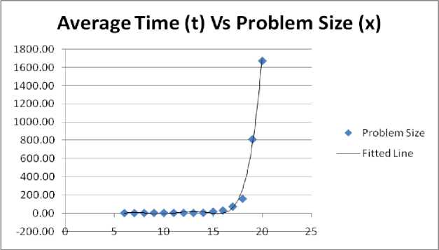
Fig. 3. Plot of Average Computational Time Vs Problem Size

It can be observed from the fitted line in Fig.3 that the computational time is polynomial of degree 6, T ( x ) = 0.002 x ⁶ - 0.132 x ⁵ + 2.614 x ⁴ - 22.51 x ³ + 59.41 x ² + 226.8 x - 1117 with the coefficient of determinant, R ² value [used to measure the goodness of fitted line], as 99%, to reach the optimal solution. However, it is observed from Table 3 and also from Fig.3 that when x >  15, the computational time grows as exponential T ( x ) = 4 x 10 ^{- 6} e ^{0.985 x} with the coefficient of determinant, R ² value, as 98%. Therefore, it can be concluded that when the total number of nodes increases, proportionally the computational time to reach the optimal solution also increases. However, almost all the problems where the input size exceeds 20 nodes, a feasible solution can be obtained with a CPU time less than 10 seconds. Therefore, this study proposes to consider using heuristic or metaheuristic algorithms to solve medium and large-scale instances to obtain a near optimal solution in a reasonable computational time.

Several different methods were employed to find a solution to VRPCD and diverse characteristics of VRP were incorporated with integrated VRPCD model in the literature. However, the operations inside a CDT are not taken into account so far. Also as per the recommendation of a literature survey [6], to focus on internal operations between indoors and outdoors of a CDT when developing the models integrating VRP and CD, VRPCD with moving shipment inside CDT is mainly considered in this study. The following aspects are taken into account in the development of VRPCD-MS model; unloading products from inbound vehicles, moving unloaded products from indoors of CDT to outdoors of CDT and loading products to outbound vehicles. Further, two different fleets of homogeneous vehicles are considered to both pickup and delivery processes separately. To solve the proposed VRPCD-MS problem, a MINLP model has been developed to minimize the total cost which includes transportation cost, loading or unloading cost, shipping cost inside CDT and vehicle operations cost. The validity of the proposed model is confirmed by the computational experiments of randomly generated fifteen small-scale instances. The proposed VRPCD-MS model was coded in LINGO (version) optimization software.

The required data such as number of inbound and outbound vehicles to complete the entire process, arrival and departure time at each node, the ready time to start the delivery process and finishing time of the entire process are obtained from LINGO output. Moreover, optimal solution of each of the fifteen tested problems and the average computational time of 10 replicates of each problem are recorded. It concludes that, the convergence rate of the problems rises to polynomial with degree 6 [ T ( x ) = O ( x ⁶) ]. Also, the study shows that for moderately large and large scale problems the computational time to reach the optimal solution is exponential [ T ( x ) = O ( e x ) ]. Since, the optimal solutions to the small-scale instances can be obtained in a few seconds of computational time, it can be concludes that this model can be used for last minute planning for similar size problems. However, the study further reveal that the optimal solution cannot be obtained in relatively less computational time for the case for medium and large-scale instances. Therefore, this study recommends for future work that to investigate the efficiency of heuristic or metaheuristic approach to obtain near optimal solutions to medium and large-scale instances. Moreover, it is recommended for further studies that to amend additional constraints to facilitate on temporary storage capacity at CDT, available vehicles to transport products, budget for components of total cost to make it more applicable to real world problems.

Acknowledgements

This research did not receive any specific grant from funding agencies in the public, commercial, or not-for-profit sectors.