Optimization of process parameters using grey-taguchi method for software effort estimation of software project

Published Online September 2018 in MECS

Software quality plays a vital role during the project development life cycle. From the customer point of view quality is important because the quality of the product is affected by the degree of customer satisfaction during the usage of the product [1]. Cost is another important parameter for developing the products. If the developed product cost is less than the market price, then the retailer industries make more profit. Hence quality and productivity are the main challenges for any company. But in many cases quality and productivity tend to be inversely proportional. So, this problem can be solved by setting the process parameters to maintain the quality. Hence, the process parameters are required to be optimized simultaneously.

In this context, much of the research has been carried out on the optimization of process parameters for various projects. GST is recently developed for system engineering theory established by Deng J [2], it is well suited in different domains namely image processing, mobile communication, decision making and system control etc. The increasing applications of GST in various fields prompted the authors to develop into its application to software effort estimation. Grey Relational Analysis (GRA) is a popular method in Grey System Theory (GST) [3]. The grey relational analysis has been applied to optimize the quality parameters over multi objective process parameters for a given project. In this paper, Grey Relational Analysis (GRA) has been used to estimate the distance between parameters and it is used to reduce the uncertainties in the projects.

Taguchi method deals with the product design in which process and product optimizations are used to improve the product quality and also reduce the cost. As this method leads to robust and parameter design, it is also referred as robust design and parameter design. Dr.Taguchi’s first work focuses on quality engineering. The Taguchi method is used to design the process parameters in order to boost the robustness in the products [4-5]. The variants of orthogonal array (OA) are defined by fixing number of columns at different levels of the arrays termed after standard orthogonal array for dealing with projects and columns representing parameters defined for the project [6]. We suggest which levels of parameters are required to find out the minimum effort of software project. This can be proved by using Grey-Taguchi method.

• II.    Related Work

Qinbao Song was used Grey Relational Analysis to predict the effort on small dataset [7]. Sun-Jen Huang proposed combination of Grey relational analysis with genetic algorithm to estimate the effort [8]. Geeta Nagpal proposed GRA method is combined with regression techniques to estimate the effort on different datasets [9]. M.Padmaja was used GRA method to estimate the effort and compare the results with existing methods [10]. This work extended using k-means clustering method to divide into clusters and applied GRA to find the effort estimation [20]. Padmaja was used BAT algorithm to estimate the effort and compare and evaluated with other models [19].

Bose, G. K attempts Grey-Taguchi method to optimize machining parameters of Electro Chemical Grinding (ECG) while machining alumina-aluminium interpenetrating phase composites [11]. P. C. Mishra used Taguchi method and grey relational analysis during the turning process of AA 7075/SiC composite in dry and spray cooling environments to optimize multi response process parameters [12].

Saikat Kumar Kuila, used Grey-Taguchi methodology to find the optimal parameters during Abrasive Water-Jet Machining (AWJM) process [13]. Different process parameters like pressure, feed rate, standoff distance and abrasive flow at three different levels are selected for optimization with two responses, higher MRR and low Ra, by a single parametric combination.

Sumit Ra, used the application of Grey-Taguchi technique for optimum parameters in Electro-Discharge Machining (EDM) of EN45 steel tool for minimum surface roughness (SR) and minimum overcut (OC) value [14]. In this paper to optimize the parameters a combination of lowest value of peak current, highest value of pulse on time, lowest value of pulse off time and voltage are applied.

The combination of these two techniques such as Grey relational analysis and Taguchi are most widely combined to optimize the parameter values and provide better performance in different related areas [15-18].

To the best of our knowledge, Grey-Taguchi method has not been used for software effort estimation and optimization and hence this combination is applied in this paper.

• III.    Methodology

In this work, Taguchi and Gray Relational Analysis methods are to be combined. Taguchi method is used to improve the quality of the project with usage of suitable parameter levels and the GRA provides the grades for the projects from the historical projects it will be help to predict the effort of a particular project. Through this combination, this paper aims in producing better parameter sequence at different levels for estimating the cost and effort for a given project. The process of obtaining this sequence is explained in the following subsections.

• A.    Taguchi Method

The Taguchi method is used in the area of an engineering approach and a statistical method to achieve the product quality. This method was proposed by Dr. Genichi Taguchi, it is a well-organized method to improve the process/product design with help of levels of significant parameters that affect to deliver the product [5]. To tune the parameter values in this use orthogonal array (OA) design [6]. From these levels we decide which level of all parameters required to developing the product with quality.

• B.    Grey Relational Analysis (GRA)

Grey System Theory was proposed by Deng in 1980. One of the method from the system is Grey relational analysis (GRA) is selected to work on uncertain conditions. It was helped to find nearest or similar projects of develop the current project from the historical projects.

Based on similar projects choose k nearest projects and estimate the effort of a developed project with the help of Grey Relational Garades (GRG).

• a.    Normalization

In order to develop the project, customer can provide the data dynamically, because they are not having complete idea of the product or project. The available data is converted into numeric data where priority given to all parameters equal. To avoid irregularity of parameters, data must be normalized using some methods. These methods used depend on nature of the data.

Here, Kemerer data set has been selected consisting of parameters such as duration, KSLOC and function points since they influence the effort estimation. To normalize the parameters this paper used, larger-the-better and smaller-the- better methods as shown in Equations (1) and (2).

Upper-bound effectiveness (i.e., larger – the – better):

x_i ( k )^*

x , ⁽ k ) - min x , ⁽ k ) max x₄ ( k ) - min x_t ( k )

Here i = 1,2, , , , m and k = 1,2,3, , , , n

Lower-bound effectiveness (i.e, smaller – the – better):

x ( k )^*

max Xj ( k ) - Xj ( k ) max x_t ( k ) - min x_t ( k )

Here i = 1,2, , , , m and k = 1,2,3, , , , n

Where, x ( k ) stand for the value of the k^th attribute in the i^th series;

x ( k ) ^* stand for the modified grey relational generating of the k^th attribute in the i^th series;

max x ( k ) means the maximum of the k^th attribute in all series;

min x(k) means the minim um of the kth attribute in all series;

development. As a last step experiments are conducted to improve GRG on the obtained optimal process parameters. Hence, through the application of GRA and Taguchi method some improvements on GRG are obtained as shown in the experimental results.

• b.    Grey Relational Coefficient (GRC)

In the process of GRA, to find coefficients of current project with historical projects by using Grey Relational Coefficient (GRC).

To calculate coefficients of parameters in all projects, Equation (3) was used.

GRC can be calculated as,

γ ( x ₀( k ), x_i ( k )) =

^Δ min ^{+ ζ Δ} max Δ 0 i ( k ) + ζ Δ max

Here ζ is the distinguishing coefficient. Depending on the practical requirements, the value of the distinguishing coefficient may be appropriately tuned.

ζ ∈ (0,1] i.e 0.5

Δ 0 i ( k ) = I x ₀ ( k ) - x_i ( k ) I i.e. Delta values or Deviation coefficients

Δ _min = min _i min _j I x ₀( k ), x_i ( k ) I

Δ _min = max _i max _j I x ₀( k ), x_i ( k ) I

• c.    Grey Relational Grade (GRG)

GRG is used to describe and explain the relation between two sets. GRG can be used to show the degree of similarity between the project to be estimated and its historical projects using Equation (4).

1 ⁿ

Γ ( x ₀( k ), x_i ( k )) =   ∑ γ ( x ₀( k ), x_i ( k ))       (4)

ⁿ k = 1

Where, i ϵ {1, 2, 3, , , n}, n is the number of response parameters

• d.    Grey Relational Rank (GRR)

Inorder to estimate the effort of a project, a historical project with highest GRG is to be selected among all projects [9]. Ranks should be assigned with respect to the GRG with most influenced project to find effort estimation of new project.

• C.    Grey-Taguchi Method

Grey-Taguchi method can be used for selection of optimal process parameters. GRA as a first step has been applied on experimental data to find the Grey Relational Grades (GRG). And then orthogonal arrays are used in this method to assign the levels of process parameters. Hence, a combination of GRA and Taguchi methods are used to find out the optimal parameters, naming this technique as Grey-Taguchi method. After calculating the optimal process parameters that are in sequence, ANOVA is used to analyze GRG to identify how each of the process parameter is contributing to the project

• IV. Experimental Results

To conduct experiments in this paper, a popular dataset (Kemerer dataset) was used, since it contains all the requisite parameters to deal with the efficiency of a project. The values of duration, size and different types of function points were obtained from various projects are shown in the below Table (1).

Table 1. Experimental results for output parameters of different projects

ID	Duration	KSLOC	AdjFP	RAWFP
1	17	253.6	1217.1	1010
2	7	40.5	507.3	457
3	15	450	2306.8	2284
4	18	214.4	788.5	881
5	13	449.9	1337.6	1583
6	5	50	421.3	411
7	5	43	99.9	97
8	11	200	993	998
9	14	289	1592.9	1554
10	5	39	240	250
11	13	254.2	1611	1603
12	31	128.6	789	724
13	20	161.4	690.9	705
14	26	164.8	1347.5	1375
15	14	60.2	1044.3	976
16	5	40.5	100	120

A. Normalization

Table 2. Normalization

Duration	KSLOC	AdjFP	RAWFP
0.5385	0.5221	0.5062	0.4175
0.9231	0.0036	0.1846	0.1646
0.6154	1	1	1
0.5	0.4268	0.312	0.3585
0.6923	0.9998	0.5608	0.6795
1	0.0268	0.1456	0.1436
1	0.0097	0	0
0.7692	0.3917	0.4047	0.412
0.6538	0.6083	0.6765	0.6662
1	0	0.0635	0.07
0.6923	0.5236	0.6847	0.6886
0	0.218	0.3122	0.2867
0.4231	0.2978	0.2678	0.278
0.1923	0.3061	0.5653	0.5844
0.6538	0.0516	0.4279	0.4019
1	0.0036	0	0.0105

As normalization plays a key role in achieving scalability of a project, all the parameters from the data set were normalized. To perform experimentations all, the parameters were normalized between a scale of [0, 1], because all parameters must be in between 0 and 1. To normalize ‘duration parameters’ in this work we used ‘larger the better’ method mentioned in Equation (1) and ‘smaller the better’ method using Equation (2) for the remaining values. The results of normalizing the parameters are shown in Table (2).

• B.    Grey Relational Coefficients (GRC)

The values of Deviation coefficients and grey relational coefficients with ζ = 0.5 are calculated and presented in Table (3) and Table (4) by using Equation (3).

Table 3. Deviation coefficients or Delta values

Duration	KSLOC	AdjFP	RAWFP
0.4615	0.4779	0.4938	0.5825
0.0769	0.9964	0.8154	0.8354
0.3846	0	0	0
0.5	0.5732	0.688	0.6415
0.3077	0.0002	0.4392	0.3205
0	0.9732	0.8544	0.8564
0	0.9903	1	1
0.2308	0.6083	0.5953	0.588
0.3462	0.3917	0.3235	0.3338
0	1	0.9365	0.93
0.3077	0.4764	0.3153	0.3114
1	0.782	0.6878	0.7133
0.5769	0.7022	0.7322	0.722
0.8077	0.6939	0.4347	0.4156
0.3462	0.9484	0.5721	0.5981
0	0.9964	1	0.9895

These coefficients of every parameter are initially obtained through estimating the deviations of every parameter with 1. Then coefficients of every parameter were calculated using Equation (3) as shown in Table (4).

• C.    Grey Relational Grades (GRG)

After finding the Grey Relational Coefficients (GRC) of every parameter, Grey Relational Grades (GRG) was calculated using Equation (4). Then ranks were assigned to every project as GRO. The respective GRG values and GRO’s are presented in Table (5). From the ranking of projects obtained the most influenced project that which has the highest order. From the Table (5) third project has the first rank so it is most influenced project to optimize the process parameters.

Table 5. GRG and GRO values

Project No	GRG	GRO
1	0.4991	10
2	0.4888	11
3	0.8913	1
4	0.4562	14
5	0.6901	2
6	0.5193	5
7	0.5005	9
8	0.5129	6
9	0.5896	4
10	0.5078	7
11	0.5902	3
12	0.3891	16
13	0.4238	15
14	0.4706	12
15	0.4645	13
16	0.5008	8

• D.    Orthogonal Array

  Table 4. Grey Relational Coefficients

  Duration	KSLOC	AdjFP	RAWFP
  0.52	0.5113	0.5031	0.4619
  0.8667	0.3341	0.3801	0.3744
  0.5652	1	1	1
  0.5	0.4659	0.4209	0.438
  0.619	0.9996	0.5324	0.6094
  1	0.3394	0.3692	0.3686
  1	0.3355	0.3333	0.3333
  0.6842	0.4511	0.4565	0.4596
  0.5909	0.5607	0.6072	0.5997
  1	0.3333	0.3481	0.3497
  0.619	0.5121	0.6133	0.6162
  0.3333	s0.39	0.4209	0.4121
  0.4643	0.4159	0.4058	0.4092
  0.3824	0.4188	0.5349	0.5461
  0.5909	0.3452	0.4664	0.4553
  1	0.3341	0.3333	0.3357

  
  

  Table 6. L16 Orthogonal Array

  S.No	A	B	C	D
  1	1	1	1	1
  2	1	2	2	2
  3	1	3	3	3
  4	1	4	4	4
  5	2	1	2	3
  6	2	2	1	4
  7	2	3	4	1
  8	2	4	3	2
  9	3	1	3	4
  10	3	2	4	3
  11	3	3	1	2
  12	3	4	2	1
  13	4	1	4	2
  14	4	2	3	1
  15	4	3	2	4
  16	4	4	1	3

  
  

Orthogonal Array (OA) is a statistical method of defining parameters that converts test areas into factors and levels. In this paper, a suitable orthogonal array design has been selected that suits for estimation and optimization. Also in this paper, the control parameters are fixed to a user defined value to evaluate the process performance.

Based on all parameters we apply orthogonal array by using MINITAB 16 on 16 projects. Table (6) shows L16 Orthogonal Array (OA).

Table 7. Different levels of process parameters

Process parameters	Notation	L1	L2	L3	L4
Duration	A	5	15	25	35
KSLOC	B	35	150	300	450
AdjFP	C	95	1000	1500	2400
RAWFP	D	95	1000	1500	2400

On actual data to conduct the experiments based on L16 Orthogonal Array process parameters and their corresponding levels are presented in Table (7).

• E.    Parameter Sequence

Taguchi and Grey Relational Analysis methods are applied to generate response tables for evaluating the average grey relational grade to every factor level as shown in Table (8).

Table 8. Sequence of levels of parameters for GRG

Parameters	L1	L2	L3	L4
Duration	0.5839	0.5557	0.5192	0.4649
KSLOC	0.5507	0.4966	0.6116	0.4648
AdjFP	0.5274	0.5081	0.6161	0.4721
RAWFP	0.4648	0.5039	0.6475	0.5074
Avg	0.5317	0.5161	0.5986	0.4773
	Total mean GRG = 0.5309

From Table (8), we can observe the sequence of parameters leading to the refinement of Grey Relational Grade. As seen from the Table (8), to evaluate the improvement of GRG a sequence of parameters to be considered as maximum values in all process parameters i.e. duration at Level 1 (L1=0.5839), KSLOC at Level 3 (L3=0.6116), AdjFP at Level 3 (L3=0.6161) and RAWFP at Level 3 (L3=0.6475) denoted in terms of notations as A1-B3-C3-D3 are to be considered. From the values obtained in the response table in order to develop a new project, the parameter would be considered from only those levels where the values are maximum.

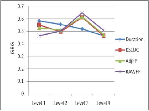
Fig.1. Main effect parameters for mean Grey Relational Grade

From the above experiment, the best process parameter levels can be considered as duration at L1, KSLOC at L3, AdjFP at L3, RAWFP at L3 as depicted in Figure (1).

• F.    Analysis of Variance (ANOVA)

ANOVA is a statistical analysis method, is generally used to examine which of the parameters significantly influence the performance characteristics. ANOVA shows the Degree of Freedom (DOF), Sum of Squares (SS), Mean Squares (MS), F value, P value and percentage of contribution of every parameter. Contributions of the parameters are calculated in percentages, deciding which parameter has the high impact contribution presented at the significant level. Finally, all contributions of parameters reach at 100% including error contribution. This is shown clearly in Table (9).

In this paper, ANOVA is applied over GRG to identify how each process parameters is contributing. Every parameter contribution is shown in Table (9). If F value is more on any parameter then contribution of that parameter is considered to be more. This can also be observed in Table (9).

Table 9. ANOVA results for performances

Process Parameters	DOF	Sum of Squares	Mean Squares	F	P	Contribution (%)
Duration	3	0.0303	0.0101	1.5075	0.8996	13.5449
KSLOC	3	0.0122	0.0041	0.6119	0.1575	5.4537
AdjFP	3	0.11	0.0367	5.4776	0.8343	49.173
RAWFP	3	0.051	0.017	2.5373	0.3031	22.7984
Error	3	0.0202	0.0067			9.03
Total	15	0.2237				100

From the above table AdjFP has more significant value is 49.17%, it is more influenced to estimate the effort, the next position on RAWFP parameter has 22.79% significant, the next position on Duration parameter is 13.54% and finally less significant value on KSLOC parameter is 5.45%. Finally, all parameter contributions including error contribution reach to 100%. If that contribution gets 100% then receive accurate results. We proved from the ANOVA method, it is shown in above Table (9).

• G.    Experimental Result

The optimal levels of parameters are indicated based on results as presented in Table (8). From these levels, GRG is estimated in subsequent experiments using Equation (5).

y = Y_m + Z ?=i (Y_/-Y_m)         (5)

Here Y is the estimated GRG

Ym is the total average GRG

• Y_; is the men of GRG at the optimal level

And n is the number of process parameters

Table 10. Comparisons on process parameters using initial level to optimal level

Parameters	On initial levels	Required levels
		Prediction	Experiment
Sequence	A1-B4-C4-D4	A1-B3-C3-D3	A1-B3-C3-D3
Duration	18	10.9375	15
KSLOC	214.4	429.9438	450
AdjFP	788.5	2197.744	2306.8
RAWFP	881	2192.25	2284
GRG	0.4562	0.8663	0.8913
	Improvement  in  GRG  is 0.4351

The prediction values of optimal process parameters can be calculated by using optimal parameters on L16 orthogonal array with GRG’s. Then every parameter from the initial process parameter is compared to predicted process parameters. It can be noticed that duration is minimum on predicted duration. Similarly, larger values are obtained on various parameters are size, AdjFP and RAWFP from initial process parameters to optimal process parameters. All parameters can be satisfied on the initial process parameters to predicted process parameters. This can be shown in Table (10). It is found that the improvement in the grey relational grade is 0.4351 from the initial parameters to optimal parameters through experiment. When this is followed the optimized process parameters such as Duration, KSLOC and function points as specified by Grey-Taguchi method there is chance to minimize the effort of software project.

• V. Conclusion and Future Work

In this paper, the process parameters are optimized of software projects using Grey-Taguchi method. The optimized process parameter sequence at different levels generated in the empirical results proves that the proposed method is favorable. Also this work proves that the parameters that exhibit higher contribution value are the most significant parameters in project design. Finally, the feasibility of Grey-Taguchi method has been proven as best in solving multi-response optimization problems.

The extension of the proposed work can be done by applying the same mechanism on different datasets to obtain optimized parameter levels which helps in estimating effort effectively.