Optimizing Knapsack Problem with Improved SHLO Variations

1.    Introduction and Related Work

Optimizing constrained combinatorial optimization problems is a challenging problem. These problems are difficult due to huge search space. The 0/1 knapsack problem is one of the important problems reported in the literature. The 0/1 Knapsack Problem is a classic representation of resource allocation challenges. Solutions derived from advanced algorithms not only benefit theoretical problem-solving but also have practical applications in resource management. This is crucial in operations research, where efficient resource allocation can lead to cost savings, improved processes, and streamlined workflows. In operations, effective supply chain management is contingent on optimal decision-making. Algorithms that excel at solving combinatorial optimization problems like the Knapsack Problem contribute directly to enhancing supply chain efficiency. This has implications for industries relying on intricate supply chain networks, such as manufacturing and logistics. Solving complex optimization problems aids in the development of decision support systems. These systems are invaluable in operations research, providing decisionmakers with data-driven insights into resource utilization, inventory management, and overall operational efficiency. The problem is a common non-polynomial problem in operations research [1]. In literature, applications of 0/1 knapsack problem were mentioned in different domains such as cryptosystem [2] and optimal load shedding [3]. Numerous disciplines such as operations research, resource allocation, economics and genetics contain applications of this problem. Finding the combination of items that produce the highest total profit while staying within the weight restriction is the difficult part. The problem definition is as follows. The problem at hand is known as the “Knapsack Problem”. It involves a set of ‘p’ items, each characterized by its weight (WTj) and profit (PIj). The objective is to determine the optimal selection of items to maximize the total profit (see equation 1), while adhering to the constraint that the combined weight of the selected items should not exceed the capacity ‘C’ of the knapsack. The decision variable, ‘Zj’, represents the selection status of the jth item, where ‘Zj’ takes binary values (0 or 1). A value of ‘1’ for ‘Zj’ indicates that the jth item is selected and included in the knapsack, while a value of ‘0’ means the item is not selected.

Maximize:

∑ PI j Z j for j from 1 to p                                         (1)

Subject to

∑ WT j Z j ≤ C where Z i ∈ { 0,1 }

The 0/1 Knapsack Problem is used in various real-world applications:

• •    Efficiently allocate limited resources in project management.

• •    Optimize investment portfolios with risk and return objectives.

• •    Minimize waste in manufacturing and supply chain management.

• •    Feature Selection in Machine Learning

• •    Optimize data transmission in broadcasting and telecommunications.

• •    Handle multiple conflicting objectives in optimization.

• •    Packing items into bins with limited capacity.

The problem's NP-hardness arises from the exponential number of possible combinations of items that can be chosen for the knapsack. Therefore, traditional brute-force approaches become computationally intractable for large instances. To solve the 0/1 Knapsack Problem efficiently, dynamic programming is a common approach. The dynamic programming algorithm builds a table, often called the “knapsack table,” to store the intermediate solutions for subproblems. By iteratively evaluating and updating the table, the algorithm finds the optimal combination of items that maximizes the total value within the knapsack's weight capacity.

The 0/1 Knapsack Problem is NP-hard, representing a class of computationally challenging problems. Developing effective algorithms to solve such problems contributes to the broader field of algorithmic advancements. Techniques and insights gained from tackling the Knapsack Problem can be applied to other optimization challenges, fostering innovation in algorithm design. Several techniques, such as greedy algorithms and metaheuristics like genetic algorithms and simulated annealing, can also be applied to approximate solutions for the 0/1 Knapsack Problem. The 0/1 knapsack problem is studied and experimented with different exact and metaheuristic algorithms. The problem is a constrained combinatorial optimization problem that makes it NP. The complexity increases with the size of the problem. In literature, the problem is investigated with algorithms such as simulated annealing (SA) [4], flower pollination algorithm [5], genetic algorithms (GAs) [6,7], ant colony optimization (ACO) [8,9], particle swarm optimization (PSO) [10,11], harmony search (HS) [12,13] and the exact methods [14,15,16]. In addressing the 0/1 Knapsack Problem, a paper proposed an Improved Simulated Annealing (SA) algorithm. The focus was on efficient problem-solving by extracting optimal and near-optimal solution spaces, addressing issues associated with the Metropolis rule in SA [4]. Another study aimed to enhance the Flower Pollination Algorithm (FPA) by introducing variations influenced by genetic algorithms. Three versions, incorporating crossover and mutation concepts, showed effectiveness, particularly for smaller instances of the 0/1 Knapsack Problem [5]. The authors proposed a Guided Genetic Algorithm (GGA) for the Multidimensional Knapsack Problem (MKP). By optimizing item-to-knapsack assignments, GGA demonstrated significant improvement over standard Genetic Algorithms (GA) [6]. In the realm of fuzzy environments, an Improved Genetic Algorithm (GA) addressed the constrained knapsack problem with discounts. Refining and repairing operations enhanced the algorithm's effectiveness under fuzzy conditions [7]. Ant Colony Optimization (ACO) was adapted for the 0/1 Knapsack Problem, emphasizing differences with the traveling salesman problem. Improved parameters showcased the robustness and potential power of this meta-heuristic algorithm [8]. An innovative ACO algorithm, combining inner and outer mutation strategies, was proposed for the knapsack problem. The model demonstrated better solutions, showcasing the algorithm's exploration and exploitation capabilities [9]. For challenging knapsack problems, a Binary Particle Swarm Optimization (BPSO) algorithm, modified for discrete space, outperformed existing approaches. It demonstrated efficacy in handling hard optimization problems [10]. The Greedy Particle Swarm Optimization (GPSO) emerged as an efficient method for the knapsack problem. Combining a greedy transform method with binary particle swarm optimization showcased improved exploration and convergence [11]. The Harmony Search (HS) algorithm found application in solving single and multi-objective knapsack problems. HS demonstrated optimal results, particularly for smaller instances, emphasizing its exploration and exploitation capabilities [12]. A novel Global Harmony Search algorithm, incorporating position updating and genetic mutation, proved efficient for 0–1 knapsack problems. Computational experiments showcased its robustness and potential in combinatorial optimization [13]. A branch-and-bound approach addressed the Knapsack Problem with Conflict Graph (KPCG), efficiently selecting a maximum profit set while considering incompatibilities. The method showcased superior efficiency for instances with a graph density of 10% and larger [14]. Extending the classical 0-1 knapsack problem with disjunctive constraints, pseudopolynomial algorithms efficiently solved the Knapsack Problem with Conflict Graph. The proposed algorithms provided effective solutions for specific graph structures [15]. A new exact algorithm efficiently solved the Multiple Knapsack Problem (MKP), especially for large instances. The algorithm showcased stable and efficient performance, highlighting its suitability for practical applications [16].

Metaheuristic algorithms are utilized when an approximate solution to a problem is sufficient and the exact solution is expensive. Although metaheuristic algorithms sometimes produce optimal results and other times near-optimal results, metaheuristics do not always result in the best solution. It is currently an active topic in the evolutionary computation community to design algorithms to optimize solutions. Similar to other biologically inspired and naturally inspired algorithms, the SHLO is inspired by the learning mechanism of humans [17]. Human learns better through repetition and it is optimized with respect to the iterations. Human learning optimization is popular due to its simple steps and high global search capability. The main objective of the paper is to design efficient human learning optimization for solving small and large instances of 0/1 knapsack problems. Contributions of the paper are:

• •    Designed variations of a metaheuristic algorithm based on “human learning optimization” to solve small and large instances of the 0/1 Knapsack Problem efficiently.

• •    Introduced three distinct “exploration capabilities” variants of the human learning optimization algorithm tailored for solving the 0/1 Knapsack Problem.

• •    The results demonstrated that all proposed variants consistently outperformed on small datasets, providing optimal solutions. Notably, Variation 2 and Variation 3 showed the best performance across both small and large datasets, significantly reducing the computational time required for problem-solving. This reduction in computational time is particularly crucial for handling larger instances of the problem, enhancing the algorithm's practical applicability.

2.    Simple Human Learning Optimization Algorithm

Section 2 describes the details of the simple human learning optimization and proposed variations for solving 0/1 knapsack problem. Section 3, presents four datasets, obtained results and comparison of proposed algorithms. Section 4 is conclusion.

Reasoning, which is a crucial component of many human cognitive processes, enables us to better understand situations and improve our learning capacity. The concept of reasoning along with human learning optimizations is presented by [18]. The effectiveness of simple human learning can be enhanced through competition and collaboration, which are two fundamental forms of social cognition. These forms encourage people to learn more effectively and solve problems more quickly by stimulating their competitive nature and fostering social engagement [19]. An adaptive simplified HLO is proposed in the paper [20] uses an adaptive strategy. The algorithm utilizes various learning parameters to implement learning from different learning strategies. To improve the exploration capacity and efficiency additional operators like random exploration learning operator and relearning operators are introduced [21].

A single individual is represented as a binary string. Since every human start learning with no prior knowledge of the problem hence these individuals are initialized with ‘0’ and ‘1’ randomly. The single bit of the binary string represents a basic bit of knowledge that an individual learned from the different modes of learning which helped the individual in problem-solving.

Population = [ a 1 , a 2 , a 3 ,... a s ]

where ‘S’ is population size.

aPq e {0,1} where 1 < p < S and 1 < q < L apq is the qth bit of the pth individual. ‘S’ is size of the population and ‘L’ denote the length of solutions.

Simple Human Learning Optimization algorithm uses three learning operators namely random, individual and social that generate new solutions. The individual learning operator and social learning operator use knowledge stored in the IKD and SKD respectively. Paper [17] presented the use of two algorithmic parameters namely “pr” and “pi” for deciding probabilities of three operators. The algorithm chooses the learning mode for each bit updation randomly based on values of “pr” and “pi” . If the randomly generated number is between 0 and “pr” then the random learning operator is called. The random number in between “pr” and “pi” shows individual learning. Randomly number higher than “pi” shows social learning. This sub-section presents variations in SHLO based on the new solution generation step.

The Pseudocode of the Simple Human Learning Optimization algorithm is given below.

SHLO Pseudocode

Function SHLO (PopulationSize, TerminationCondition, pr, pi)

Population = InitializePopulation(PopulationSize)

IKD = InitializeIKD()

SKD = InitializeSKD()

While Not TerminationConditionReached

CalculateFitness(Population)

NewPopulation = GenerateNewPopulation(Population, IKD, SKD, pr, pi)

CalculateFitness(NewPopulation)

UpdateKnowledgeBase(IKD, SKD, Population, NewPopulation)

Population = NewPopulation

End While

End Function

Function GenerateNewPopulation (Population, IKD, SKD, pr, pi)

NewPopulation = EmptyPopulation()

For Each Individual in Population

For Each Bit in Individual

Operator = SelectLearningOperator(pr, pi)

If Operator is RandomLearning

NewBit = RandomLearningOperator()

Else If Operator is IndividualLearning

NewBit = IndividualLearningOperator(IKD, Individual)

Else If Operator is SocialLearning

NewBit = SocialLearningOperator(SKD)

SetBitInNewIndividual(NewPopulation, NewBit)

End For

End For

Return NewPopulation

End Function

Function RandomLearningOperator()

• // Equation 2: Random learning operator

If RandomNumber() ≤ 0.6

Return 0

Else

Return 1

End If

End Function

Function IndividualLearningOperator(IKD, Individual)

• // Equation 4: Individual learning operator

RandomSolution = RandomlySelectSolution(IKD)

Return BitFromSolution(RandomSolution)

End Function

Function SocialLearningOperator(SKD)

• // Equation 5: Social learning operator

RandomSolution = RandomlySelectSolution(SKD)

Return BitFromSolution(RandomSolution)

End Function

Function UpdateKnowledgeBase(IKD, SKD, Population, NewPopulation)

UpdateIKD(IKD, Population, NewPopulation)

UpdateSKD(SKD, NewPopulation)

End Function

Random learning operator: This operator updates the values in a random fashion. It indicates that no prior knowledge is required to generate new solution. It provides a straightforward but effective way for people to experiment with new ideas and enhance their learning. The random learning operator is presented in equation 2. The bit is updated to value ‘0’ is the random number generated is less than 0.6 else value ‘1’.

a j = RLO {^ ^6}

Individual learning operator: It allows independent problem-solving. Being able to autonomously speculate about problems while learning is a beneficial learning skill. The individuals can use the individual learning technique to learn from their prior knowledge and experience, which helps them to avoid mistakes and increase learning effectiveness. The Individual Knowledge Database (IKD) keeps a record of the best individual experiences with the highest fitness values for individual learning.

Social learning operator: Some problems can be solved by humans alone. However, when dealing with complex problems, relying solely on random and individual learning modes might not be as effective. The social learning hypothesis suggests that social learning plays a crucial role in human learning, as knowledge sharing within a social setting can significantly enhance learning effectiveness. Previous research shows that humans instinctively learn through imitation and can acquire a great deal by emulating the good examples set by their siblings, elders, idols, and teachers. In such situations, knowledge and skills are transmitted among individuals, either directly or indirectly, leading to improved learning efficiency and effectiveness through the sharing of experiences. To replicate this effective learning approach, the population's knowledge is stored using the Social Knowledge Database (SKD).

	гa		Г a il	a12	a1]	'   air
	a2		a2i	a22	•   a2j   •	•   «2*
Knowledge Database —	a‘	-	a i	ai2    •	aij	'    atl	(3)
			asi	as2	asj

Equation 3 represents the general structure of the database for both IKD and SKD. In the case of IKD, ‘S’ represents the number of previous solutions of each individual in the population. In the case of IKD, a_i represents i^th solution from IKD for an individual and a_i j indicates the ikd_i j i.e. the j^th bit of i^th solution from IKD. Equation 4 shows that j^th bit from the binary individual ‘ a’ is replaced by the j^th bit of the ‘b^th’ solution from IKD of i^th individuals.

a y = ikd bj                                                  (4)

SKD solutions contain the global best solutions. When SKD is used the solutions will be the global best experience instead of the individual’s personal best experiences. Similar to IKD, SKD is implemented by using equation 5.

a iy = skd by                                                    (5)

where skd ij suggests i^th bit of b^th solution from SKD.

3.    Proposed SHLO Variations 3.1    Variation 1 (V1): Learning Mode Constraint

In this particular variation, the learning mode for individuals is constrained, which means that they do not select learning modes independently for each bit in their solutions. Instead, an individual in the current iteration of the algorithm learns from only one specific mode of learning. To generate a new solution, the individual replaces the entire binary string according to a single learning strategy. Unlike other variations where each bit can be influenced by different learning modes, here the individual adheres to a single learning approach for the entire solution.

For example, if the chosen learning mode is “random learning,” the new solution is generated by stochastically replacing all bits with either ‘0’ or ‘1’. The stochastic replacement implies that each bit has a certain probability of being set to '0' or '1' based on the random process. This generates diversity in the new solutions, as different combinations of bits are explored during the replacement process.

Function GenerateNewPopulation_V1(Population, IKD, SKD, pr, pi)

NewPopulation = EmptyPopulation()

For Each Individual in Population

LearningMode = SelectLearningMode(pr, pi)

NewIndividual = GenerateNewIndividual_V1(Individual,

LearningMode, IKD, SKD)

AddToPopulation(NewPopulation, NewIndividual)

End For

Return NewPopulation

End Function

Function GenerateNewIndividual_V1(Individual, LearningMode, IKD,

SKD)

NewIndividual = EmptyIndividual()

For Each Individual

If LearningMode is RandomLearning

NewIndividual = RandomLearningOperator()

Else If LearningMode is IndividualLearning

NewIndividual = IndividualLearningOperator(IKD, Individual)

Else If LearningMode is SocialLearning

Individual = SocialLearningOperator(SKD)

End For

Return NewIndividual

End Function

The GenerateNewPopulation_V1 function aimed to create a new population by generating new individuals based on the current population, individual knowledge domains (IKD), and social knowledge domains (SKD). For each individual in the population, it selected a learning mode using probabilities (pr and pi) and then generated a new individual using the GenerateNewIndividual_V1 function. This new individual was added to the new population. The GenerateNewIndividual_V1 function created a new individual by iterating through the bits of the existing individual and applying a learning operator based on the selected learning mode, which could be random learning, individual learning, or social learning.

By restricting individuals to a single learning mode for each iteration, this variation can explore the solution space in a more focused manner and may be particularly effective when the problem exhibits specific patterns or characteristics that align with the chosen learning strategy. However, it also means that other learning modes are not utilized for generating new solutions in that particular iteration.

Equation 6 shows how the solution will be updated in case of individual and social learning. The ith solution is replaced by the yth solution from IKD and similarly in the case for SKD.

a i = ikd y (6)

• V1 tends to focus on a more targeted exploration. Restricting individuals to learn from only one specific mode for the entire solution in a given iteration, emphasizes a depth-first approach. The constrained learning mode can be advantageous when there are patterns or characteristics in the problem that align with the chosen learning strategy. It allows individuals to thoroughly explore a specific aspect of the solution space. While exploration is targeted, there might be limitations in exploiting diverse strategies. Since each individual adheres to a single learning approach, there might be a risk of overlooking potentially beneficial regions of the solution space that align with different learning modes.

• 3.2    Variation 2 (V2): Intentional Bit Changes for Diversity

In this particular variation of the algorithm, a certain percentage of bits in the binary string undergo changes during the generation of a new population. This intentional alteration serves two main purposes: first, to create diversity within the population, ensuring that different solutions are explored, and second, to improve the chances of finding better solutions by exploring different regions of the solution space.

The GenerateNewPopulation_V2 function was designed to generate a new population by creating new individuals from the existing population with a specified change percentage. For each individual in the population, it generated a new individual using the GenerateNewIndividual_V2 function. This function iterated through each bit of the individual and, with a probability defined by ChangePercentage, applied a simultaneous learning operator based on IKD and SKD. If the random number exceeded the change percentage, the bit remained unchanged. The new individual was then added to the new population.

Function GenerateNewPopulation_V2(Population, IKD, SKD, pr, pi, ChangePercentage)

NewPopulation = EmptyPopulation()

For Each Individual in Population

NewIndividual = GenerateNewIndividual_V2(Individual, IKD, SKD,

ChangePercentage)

AddToPopulation(NewPopulation, NewIndividual)

End For

Return NewPopulation

End Function

Function GenerateNewIndividual_V2(Individual, IKD, SKD,

ChangePercentage)

NewIndividual = EmptyIndividual()

For Each Bit in Individual

If RandomNumber() ≤ ChangePercentage

NewBit = SimultaneousLearningOperator(IKD, SKD)

Else

NewBit = Bit

End If

SetBitInNewIndividual(NewIndividual, NewBit)

End For

Return NewIndividual

End Function

The learning process in this algorithm is unique in that it involves all three modes of learning simultaneously. These modes are referred to as the random learning operator, individual learning operator, and social learning operator. Each new solution that is generated learns from all three modes of learning. This simultaneous learning from multiple modes is achieved by dynamically selecting the learning mode for each bit every time a new solution is created.

To update the bits during the learning process, equations 2, 4, and 5 are utilized. These equations define the rules or mechanisms for adjusting the values of the bits based on the information learned from the different learning modes. The application of these equations ensures that the algorithm effectively combines the insights gained from each learning mode to improve the quality of solutions and adapt to the problem's characteristics.

• V2 introduces intentional changes to a subset of bits, promoting a broader exploration. This intentional diversity aims to explore different regions of the solution space by allowing a certain percentage of bits to be altered during the generation of new solutions. Learning from all three modes simultaneously contributes to a more comprehensive exploration strategy. By allowing intentional alterations in a subset of bits, V2 strikes a balance between exploration and exploitation. It ensures that the algorithm explores diverse solutions while still retaining information from the existing knowledge base.

• 3.3    Variation 3 (V3): Hybrid Approach - Diversity with Consistency

Variation 3 presents a hybrid approach, combining the characteristics of both variation 1 and variation 2. Like variation 2, it involves changing a certain percentage of bits in the binary string during the generation of new solutions. This intentional modification of bits aims to inject diversity into the population, allowing for the exploration of different solution regions. However, similar to variation 1, variation 3 restricts the learning mode for individuals in the current iteration. Instead of selecting learning modes independently for each bit, individuals learn from only one mode of learning, chosen from the three available options (random learning, individual learning, and social learning). With this approach, variation 3 generates a new population that exhibits some diversity while ensuring that individuals follow a specific learning strategy consistently. This combination of individual learning modes in the population can provide a balanced exploration-exploitation trade-off during the optimization process. To update the bits during the learning process, equations 2, 4, and 5 are employed. These equations define the rules for adjusting the values of bits based on the insights gained from the learning mode selected for each individual.

The GenerateNewPopulation_V3 function combined aspects of the first two versions. It generated a new population by creating new individuals from the existing population, incorporating learning modes and a change percentage. For each individual in the population, it selected a learning mode using probabilities (pr and pi) and generated a new individual using the GenerateNewIndividual_V3 function. This function iterated through each bit of the individual and, with a probability defined by ChangePercentage, applied a learning operator based on the selected learning mode, which could be random learning, individual learning, or social learning. If the random number exceeded the change percentage, the bit remained unchanged. The new individual was then added to the new population.

Function GenerateNewPopulation_V3(Population, IKD, SKD, pr, pi, ChangePercentage)

NewPopulation = EmptyPopulation()

For Each Individual in Population

LearningMode = SelectLearningMode(pr, pi)

NewIndividual = GenerateNewIndividual_V3(Individual, LearningMode, IKD,

SKD, ChangePercentage)

AddToPopulation(NewPopulation, NewIndividual)

End For

Return NewPopulation

End Function

Function GenerateNewIndividual_V3(Individual, LearningMode, IKD, SKD, ChangePercentage)

NewIndividual = EmptyIndividual()

For Each Bit in Individual

If RandomNumber() ≤ ChangePercentage

If LearningMode is RandomLearning

NewBit = RandomLearningOperator()

Else If LearningMode is IndividualLearning

NewBit = IndividualLearningOperator(IKD, Individual)

Else If LearningMode is SocialLearning

NewBit = SocialLearningOperator(SKD)

Else

NewBit = Bit

End If

SetBitInNewIndividual(NewIndividual, NewBit)

End For

Return NewIndividual

End Function

Variation 3 offers a unique compromise between diversity and consistency, leveraging the strengths of variation 1 and variation 2 to potentially achieve improved performance and convergence characteristics for solving the 0/1 Knapsack Problem.

V3 aims to achieve a balance between exploration and consistency. Similar to V2, it introduces intentional changes to promote diversity. However, like V1, it restricts the learning mode for individuals in a given iteration, ensuring a certain level of consistency. This combination is designed to provide a nuanced exploration that leverages both the benefits of intentional diversity and focused learning. By consistently following a specific learning strategy within an iteration, V3 maintains a level of exploitation. This can be beneficial when the problem exhibits characteristics that align with a specific learning mode. It aims to strike a balance between exploring new regions and exploiting known strategies.

4.    Results and Discussion

In this section, we present the dataset used in the study, followed by a concise overview of the main results and findings. Moving on to the results, key findings are summarized, highlighting significant patterns and trends.

Small dataset: Dataset 1 is taken from [22] which contains eight instances. Dataset 2 has 10 instances which are taken from [23]. Dataset 3 has 25 instances which varies from 8 objects to 24 objects which is taken from [24].

Large dataset: Dataset 4 is prepared as per guidelines from [13]. Its object weights range from 5 to 20. The object profits range from 50 to 100. The weight capacity C is {1000, 2400, 4000, 6000, 8000, 10000, 14000, 16000}.

In this study, the performance of the Simple Human Learning Optimization (SHLO) technique and its variations is evaluated using 10 repetitions for each instance from the given datasets. The obtained results are then compared against known optimal solutions and the results of other metaheuristic algorithms from previous literature. The comparison is done based on two key measures: the best-known solution achieved and the success rate. Tables 1, 2, and 3 present the comprehensive comparison of the obtained solutions of SHLO and its variations with the known optimal solutions, as well as the Harmony Search Algorithm [12] and the Flower Pollination Algorithm [5]. Overall, the results from the tables provide a comprehensive evaluation of the different SHLO variations, showcasing their strengths and weaknesses in comparison to other algorithms and their respective exploration capabilities. These findings contribute valuable insights into selecting the most suitable SHLO variation for tackling the 0/1 Knapsack Problem and provide a better understanding of their potential applications in real-world scenarios.

The results in table 1 reveal that for all instances in Dataset 1, SHLO, proposed variation V2, and proposed variation V3 successfully attain the optimal solutions. However, SHLO variation V1 fails to find the optimal solution for instance P7, indicating a limitation in its performance for that specific instance.

Table 1. Results comparison for dataset 1

Instance	Optimal	HS [12]	FPA [5]	FPA V3 [5]	SHLO	SHLO V1	SHLO V2	SHLO V3
P1	309	309
P2	51	51
P3	150	150
P4	107	107
P5	900	900
P6	1735	1735
P7	1458	1458	1458	1451	1458	1453	1458	1458

Table 2. Results comparison for dataset 2

Instance	Optimal	HS [12]	FPA [5]	FPA V3 [5]	SHLO	SHLO V1	SHLO V2	SHLO V3
p2-1	295	295
p2-2	1024	945	1024	987	1024	978	1024	1024
p2-3	35	35
p2-4	23	23
p2-5	481.06	481.06
p2-6	52	52
p2-7	107	107
p2-8	9767	9731	9712	9747	976     \	9750	9756	9755
p2-9	130	130
p2-10	1025	889	1025	1014	1025	992	1025	1025

Table 2 demonstrates that the performance of SHLO variations V2 and V3 is slightly superior to that of the Harmony Search Algorithm and the Flower Pollination Algorithm. This indicates that these SHLO variations exhibit competitive performance in comparison to these benchmark algorithms. Similarly, as shown in table 3, SHLO and its proposed variations V2 and V3 outperform the Flower Pollination Algorithm and its variations significantly. These results demonstrate the effectiveness of the SHLO techniques for solving the 0/1 Knapsack Problem and their ability to achieve better solutions than the Flower Pollination Algorithm. The comparison in tables 2 and 3 highlights that the exploration capability of SHLO variation 1 is limited, resulting in its lower performance compared to the other SHLO variations. This observation suggests that the modifications introduced in variations V2 and V3 have enhanced the exploration capacity of the algorithm, leading to improved performance and better solutions.

In table 4, a comprehensive comparison of the solutions obtained by the Simple Human Learning Optimization (SHLO) algorithm and its variations is presented for instances in dataset 4. The findings from table 4 highlight the importance of exploration capability in optimization algorithms, especially for tackling large and complex problem instances. Unlike the first three datasets, the instances in dataset 4 are characterized as large, which means they are more complex and have a higher number of objects or variables. The results in table 4 demonstrate that SHLO variation V3 outperforms both the original SHLO algorithm and the proposed variations V1 and V2 significantly. This indicates that Variation V3 achieves solutions that are of higher quality or closer to the optimal solutions, making it the most effective approach among the considered SHLO variations for solving large instances in dataset 4.

The comparison reveals that SHLO variation V1 exhibits a limited exploration capability, resulting in its lower performance when compared to both the original SHLO algorithm and the other SHLO variations. This limitation hampers the ability of variation V1 to explore diverse regions of the solution space, which may prevent it from finding better solutions, particularly for large and complex instances like those in dataset 4. SHLO variation V3 emerges as the most promising choice, demonstrating superior performance and emphasizing the significance of effective exploration strategies in solving the 0/1 Knapsack Problem efficiently.

The success rate of SHLO and its three variations is 100 percent for all instances of dataset 1. The success rate of SHLO, variation V2 and variation V3 is 100 percent for all instances except one instance namely p2-8 of dataset 2. The SHLO and all variations show a 100 percent success rate for instances from “8a” to “16e” from dataset 3. Table 5 shows the success rate of SHLO and its variations for instances from “20a” to “24e” of dataset 3. Proposed variations SHLO V1 is not suitable to solve large problem instances of dataset 3. Results presented in table 5 show that proposed variations V2 and V3 are significantly better than SHLO.

Table 3. Results comparison for dataset 3

Instance	Optimal	HS [12]	FPA [5]	FPA V3 [5]	SHLO	SHLO V1	SHLO V2	SHLO V3
8a	3924400	3924400
8b	3813669	3813669
8c	3347452	3347452
8d	4187707	4187707
8e	4955555	4955555
12a	5688887	5688887
12b	6498597	6498597
12c	5170626	5170626
12d	6992404	6992404
12e	5337472	5337472
16a	7850983	7850983	7850983	7823318	7850983	7832023	7850983	7850983
16b	9352998	9352998	9132010	9138620	9352998	9352998	9352998	9352998
16c	9151147	9151147	9111941	9051752	9151147	9151147	9151147	9151147
16d	9348889	9348889	9348889	9266369	9348889	9348889	9348889	9348889
16e	7769117	7769117	7769114	7725775	7769117	7769117	7769117	7769117
20a	10727049	10727049	10567407	10581901	10727049	10683213	10727049	10727049
20b	9818261	9818261	9638584	9673100	9818261	9753214	9818261	9818261
20c	10714023	10714023	10531375	10503619	10714023	10652375	10714023	10714023
20d	8929156	8929156	8837509	8839607	8929156	8893733	8929156	8929156
20e	9357969	9357969	9300514	9218972	9357969	9351063	9357969	9357969
24a	13549094	13549094	13284741	9218972	13549094	13408172	13549094	13549094
24b	12233713	12233713	12121436	12121436	12233713	12111122	12233713	12233713
24c	12448780	12448780	12285798	12216778	12448780	12367533	12448780	12448780
24d	11815315	11815315	11660115	11522381	11815315	11706758	11815315	11815315
24e	13940099	13940099	13733826	13381600	13940099	13876812	13940099	13940099

Table 4. Results comparison for dataset 4

Data Instance	SHLO	SHLO V1	SHLO V2	SHLO V3
kp100_1	6197	5085	6229	6447
kp100_2	6455	5347	6345	6658
kp200_1	12488	9628	12425	14814
kp200_2	12121	9345	12186	13789
kp400_1	22080	18158	22200	24349
kp400_2	21983	18158	22263	24403
kp600_1	31074	25750	31060	37598
kp600_2	30699	25983	30964	38212
kp800_1	39623	33499	40090	48915
kp800_2	40774	33718	40314	50382
kp1000_1	49033	41891	49308	61915
kp1000_2	48859	41668	48748	62821
kp1200_1	57841	50005	58019	83504
kp1200_2	57697	50257	58164	84810
kp1500_1	70256	61221	71121	100091
kp1500_2	69566	61187	70570	100167

Table 5. SHLO success rates on dataset 3

Instance	SHLO	SHLO V1	SHLO V2	SHLO V3
20a	40	0	80	100
20b	40	0	60	80
20c	40	0	60	80
20d	20	0	80	80
20e	40	0	40	60
24a	20	0	40	40
24b	20	0	40	60
24c	20	0	60	60
24d	20	0	20	60
24e	20	0	60	40

■ Proposed V2          Proposed V3

0        1000      2000      3000      4000      5000      6000

Iterations

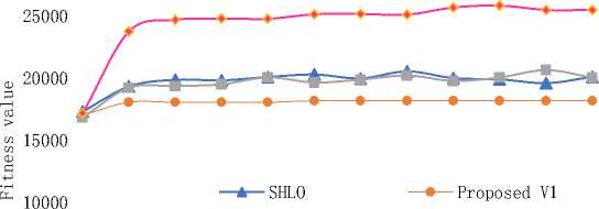
Fig. 1. Convergence for dataset instance 400_1

Iterations

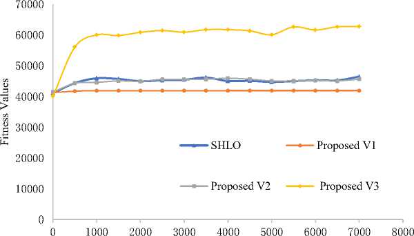
Fig. 2. Convergence for dataset instance 1000_1

Iterations

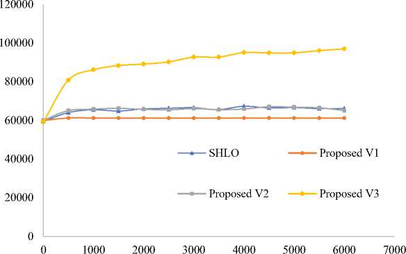
Fig. 3. Convergence for dataset instance 1500_1

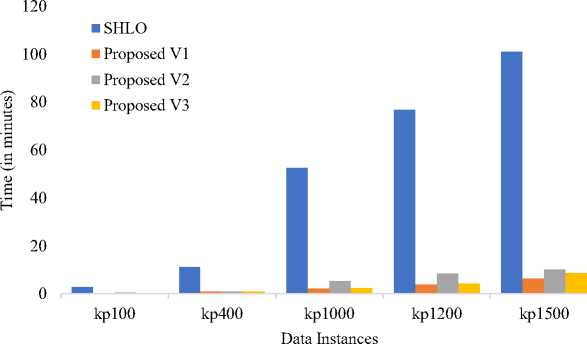
Fig. 4. Execution time on 5 data instances of dataset 4

In figure 1, 2 and 3 of the study, a comparison is presented between the performance of the Simple Human Learning Optimization (SHLO) algorithm and the proposed variations when applied to three specific instances (400_1, 1000_1, and 1500_1) from dataset 4. These instances are characterized as belonging to the large problem size category, with the number of objects in each instance being 400, 1000, and 1500, respectively.

The results from the comparison indicate interesting observations regarding the performance of the different variations. Variation 1, one of the proposed variations, demonstrates a lower exploration capacity, meaning it does not explore the solution space as extensively as the other algorithms. Consequently, it does not perform well on large datasets like the instances mentioned.

For Variation 2, the convergence speed is found to be similar to that of the SHLO algorithm. This suggests that Variation 2 is relatively competitive in terms of convergence when compared to the baseline SHLO approach.

The most significant improvement is observed in Variation 3. It outperforms the other algorithms, including SHLO and Variation 1, in terms of convergence speed. This improvement indicates that Variation 3 is able to reach high-quality solutions faster than the other methods on the mentioned large datasets.

The results from the comparison highlight the strengths and weaknesses of each algorithm in dealing with large problem instances. Variation 3 emerges as the most promising candidate due to its significant improvement in convergence speed, which can be crucial for efficiently solving complex problems.

In figure 4 of the study, a comparison of algorithms based on their execution time is presented for five sample instances taken from Dataset 4. The purpose of this comparison is to evaluate the efficiency of each algorithm in terms of the time required to complete the optimization process for these specific instances. The results from the comparison reveal that the Simple Human Learning Optimization (SHLO) algorithm exhibits significantly higher execution times when compared to the proposed variations. This indicates that SHLO takes notably longer to converge and find solutions for the given instances compared to the new variants introduced in the study. The shorter execution times observed for the proposed variations indicate improved algorithmic efficiency. This efficiency can be attributed to the modifications and enhancements made to the original SHLO algorithm in the proposed variations. These modifications might include more effective ways of exploring the solution space, faster convergence mechanisms, or other optimization techniques that contribute to the reduced execution time. The observation that the proposed variations outperform SHLO in terms of execution time is a crucial finding, especially when dealing with larger and more complex instances of the 0/1 Knapsack Problem. Reducing the execution time can lead to increased computational efficiency and enable the algorithms to tackle larger problem sizes more efficiently. The comparison in figure 4 highlights the advantages of the proposed variations over the original SHLO algorithm concerning execution time, providing valuable insights for selecting the most efficient algorithm for solving the 0/1 Knapsack Problem in practical scenarios.

The variations introduced in SHLO represent a form of algorithmic innovation in the domain of combinatorial optimization. Variation 3 (V3) consistently outperformed other variations and benchmark algorithms, demonstrating superior exploration, convergence speed, and efficiency. Variation 2 (V2) also showed competitive performance, especially in comparison to benchmark algorithms. Variation 1 (V1) demonstrated limitations, particularly in the exploration on large datasets. Combinatorial optimization problems involve making discrete decisions, and solving them efficiently is of paramount importance in various fields. The research contributes by proposing novel ways of combining learning modes and updating solution spaces, demonstrating that innovation in algorithm design can lead to more effective solutions. This aspect of algorithmic innovation is crucial for advancing the state-of-the-art in optimization and addressing the complexities of NP-hard problems. The research delves into the mechanisms of human learning and how these can be harnessed for optimization. Traditional optimization algorithms often mimic natural processes, and by specifically drawing from human learning, this research provides a unique perspective. Understanding how humans learn, adapt, and apply knowledge to problem-solving can inspire more effective algorithmic strategies. This interdisciplinary approach not only advances optimization techniques but also fosters a deeper connection between cognitive science and computational intelligence. Benchmarking is crucial in evaluating the performance of optimization algorithms. By comparing SHLO and its variations against established algorithms like the Harmony Search Algorithm and the Flower Pollination Algorithm, the research provides a comparative analysis. This benchmarking process helps identify the strengths and weaknesses of each algorithm under specific conditions. Such comparative studies are essential for guiding researchers and practitioners in choosing the most suitable algorithm for different problem types, promoting a better understanding of algorithmic behavior.

5.    Conclusion

The 0/1 Knapsack Problem, residing in the NP complexity class, has been a focal point of exploration using various exact and metaheuristic algorithms. Its inherent combinatorial constraints pose a significant challenge for efficient solutions, especially with an increase in problem size.

This research delves into the application of the Simple Human Learning Optimization (SHLO) algorithm and its three proposed variants in addressing the complexities of the 0/1 Knapsack Problem. The SHLO algorithm employs three learning operators: random, individual, and social learning. The proposed variants share these operators but diverge in their strategies for generating new solutions. Each variant introduces a unique approach to constructing a new population, involving the selection of learning operators and bits for updating. Each variation introduces a unique tradeoff between exploration and exploitation. V1 emphasizes focused exploration, V2 promotes intentional diversity for a balanced approach, and V3 combines elements of both for nuanced exploration-exploitation dynamics. The effectiveness of each variation depends on the nature of the problem and the desired balance between exploration and exploitation in the solution space.

When evaluating algorithm performance, SHLO variations V2 and V3 demonstrate superiority over the Harmony Search Algorithm and the Flower Pollination Algorithm, particularly on dataset 2 and dataset 3. Notably, for large instances in dataset 4, SHLO variation V3 outperforms SHLO, proposed variation V1, and proposed variation V2 significantly. The success rate of proposed variations V2 and V3 surpasses SHLO, indicating their effectiveness in uncovering high-quality solutions. Furthermore, the proposed variations exhibit a substantial reduction in execution time compared to SHLO, suggesting enhanced efficiency.

This study suggests avenues for further exploration, specifically in assessing the performance of SHLO and its variations in addressing the multi-dimensional 0/1 Knapsack Problem.