Optimizing Memory using Knapsack Algorithm

Author: Dominic Asamoah, Evans Baidoo, Stephen Opoku Oppong
Journal: International Journal of Modern Education and Computer Science (IJMECS) @ijmecs
Article in issue: 5 vol.9, 2017.
Free access
Knapsack problem model is a general resource distribution model in which a solitary resource is allocated to various choices with the aim of amplifying the aggregate return. Knapsack problem has been broadly concentrated on in software engineering for a considerable length of time. There exist a few variations of the problem. The study was about how to select contending data/processes to be stacked to memory to enhance maximization of memory utilization and efficiency. The occurrence is demonstrated as 0 – 1 single knapsack problem. In this paper a Dynamic Programming (DP) algorithm is proposed for the 0/1 one dimensional knapsack problem. Problem-specific knowledge is integrated in the algorithm description and assessment of parameters, with a specific end goal to investigate the execution of finite-time implementation of Dynamic Programming.
Knapsack, memory, maximization, dynamic programming, algorithm
Short address: https://sciup.org/15014969
IDR: 15014969
Text of the scientific article Optimizing Memory using Knapsack Algorithm
Published Online May 2017 in MECS
Earlier computers had a single-level scheme for memory. Computer evolution has moved from gigantic mainframes to small stylish desktop computers and to low-power, ultra-portable handheld devices with in a relatively short period of time. As the generations keep passing by, computers making up of processors, memories and peripherals turn out to be smaller and faster with memory prices going up and down. However, there has not been a single main memory that was both fast enough and large enough even though computers were becoming faster and programs were getting bigger, particularly multiple processes that were simultaneously carried out under the same computer system. Though putting more random access memory (RAM) in the computer is nearly at all times a good investment, but it is not really advisable to spend extra money to get full benefit from the memory you already have, if there is an effective algorithm to ensure effective memory utilisation.
Modern computer memory management is for some causes a crucial element of assembling current large applications. First, in large applications, space can be a problem and some technology is efficiently needed to return unused space to the program. Secondly, inexpert implementations can result in extremely unproductive programs since memory management takes a momentous portion of total program execution time and finally, memory errors becomes rampant, such that it is extremely difficult to find programs when accessing freed memory cells. It is much secured to build more unfailing memory management into design even though complicated tools exist for revealing a variety of memory faults. It is for this basis that efficient schemes are needed to manage allocating and freeing of memory by programs.
In a computer system, a process as soon as created wants to run. There is a number of N created processes all contending for memory space to run. All process want to fill the main memory that can hold an aggregate weight of W. If all processes are allowed to run, it will lead to system crushes, system running low memory, system underperformance, system overheat and difficulty in accessing data. We want to fill the main memory that can hold an aggregate weight of W with some blend of data/process from N possible list of data/process each with data size wi and priority value vi so that optimal utilisation of memory of the data/processes filled into the System main memory is achieved hence maximized.
Among the data/processes contending for memory, Which of them should be allowed to run and which should not? Does the allowable data make optimal use of memory without memory losses?
The problem that will be considered in this paper is that of accepting or rejecting the Process (an occurrence of an executed program) as they come in from the process queue to compete for memory space when a user request to run a program. The goal is to maximise the number of processes in a limited memory space.
-
II. Literature Review
Knapsack problem largely considered as a discrete programming problem has become one of the most studied problem. The motive for such attention essentially draws from three facts as stated by Gil-Lafuente et al.
-
1. It can be viewed as the simplest integer linear programming problem;
-
2. It emerges as a sub-problem in many more complex problems;
-
3. It may signify a great number of practical situations”[1].
-
A. Memory management, Processes and its allocations
The computer system primary memory management is key. After all, “all software runs in memory and all data is stored in some form of memory. Memory management has been studied extensively in the traditional operating systems field” [2]. Memory management includes giving approaches to dispense bits of memory to programs at their request, and liberating it for reuse when not really required.
Chen [3] identified possibilities of managing memory in smart home gateways. They asserts that “due to different architecture, memory management for software bundles executed in home gateways differs from traditional memory management techniques because traditional memory management techniques generally assume that memory regions used by different applications are independent of each other while some bundles may depend on other bundles in a gateway”. By way of contribution, they introduce a service dependency heuristic algorithm that is close to the optimal solution based on Knapsack problem but performs significantly better than traditional memory management algorithms and also in a general computing environment identified the difference between memory management in home gateway and traditional memory management problem.
As program advancement is shifting its way into a more extensive programming community and more conventional state-based dialects from the practical programming community, “the view that a more disciplined approach to memory management becomes a very important aspect [4]. For example, web programming languages such as Java and Python include garbage collection as part of the language, and there are various packages for performing memory management in C and C++”.
-
B. Knapsack problems and applications
The knapsack problem (KP) is a traditional combinatorial issue used to show numerous modern circumstances. “Since Balas and Zemel a dozen years ago introduced the so-called core problem as an efficient way of solving the Knapsack Problem, all the most successful algorithms have been based on this idea. All knapsack Problems belong to the family of NP-hard problems, meaning that it is very unlikely that we ever can devise polynomial algorithms for these problems” [5].
Table 1. Core history of Knapsack Problems and Solutions
|
Year |
Author |
Solution Proposed |
|
1950s |
Richard Bellman |
Produced the first algorithm - dynamic programming theory - to exactly explain the 0/1 knapsack problem. |
|
1957 |
George B. Dantzig |
He gave an exquisite and productive strategy to obtain the answer for the continuous relaxation issue, and henceforth an upper bound on z which was utilized as a part of all studies on KP in the accompanying a quarter century |
|
1960s |
Gilmore and Gomory |
Among other knapsack-type problems he explored the dynamic programming approach to the knapsack problem |
|
1967 |
Katherine Kolesar |
Experimented with the first branch and bound algorithm of the knapsack problem. |
|
1970s |
Horowitz and Sahni |
The branch and bound methodology was further created, turned out to be the main approach fit for taking care of issues with a great amount of variables. |
|
1973 |
Ingargiola and Korsh |
Presented the initial reduction formula, a pre-processing algorithm which significantly reduces the number of variables |
|
1974 |
Johnson |
Gave the first polynomial time approximation design to solve the problem of the subset-sum; Sahni extended the result to the 0/1 knapsack problem. |
|
1975 |
Ibarra and Kim |
They introduce the first completely polynomial time approximation design |
|
1977 |
Martellon and Toth |
Proposed the first upper bound taking over the charge of the continuous relaxation. |
|
The key products of the eighties concern the resolution of mass problems, for which variables cataloguing (required by all the most effective algorithms) takes a very high percentage of the running time. |
||
|
1980 |
Balas and Zemel |
Introduced another way to deal with the issue by sorting, much of the time, just a little subset of the variables (the core problem). They demonstrated that there is a high likelihood for discovering an ideal solution in the core, in this way abstaining from considering the remaining objects. |
The Knapsack problem has been concentrated on for over a century with prior work dating as far back as 1897. “It is not known how the name Knapsack originated though the problem was referred to as such in early work of mathematician Tobias Dantzig suggesting that the name could have existed in folklore before mathematical problem has been fully defined” [6].
Given a knapsack of limit, Z, and n dissimilar items, Caceres and Nishibe [7] algorithm resolved the single Knapsack problem using local computation time with communication rounds. With dynamic programming, their algorithm solved locally pieces of the Knapsack problem. The algorithm was implemented in Beowulf and the obtained time showed good speed-up and scalability [8].
Heuristic algorithms experienced in literature that can generally be named as population heuristics include; “genetic algorithms, hybrid genetic algorithms, mimetic algorithms, scatter-search algorithms and bionomic algorithms”. Among these, Genetic Algorithms have risen as a dominant latest search paradigm [9].
Eager about making use of a easy heuristic scheme (simple flip) for answering the knapsack problems, Oppong [10] offered a study work on the application of usual zero-1 knapsack trouble with a single limitation to determination of television ads at significant time such as prime time news, news adjacencies, breaking news and peak times.
-
C. Related Works
The Knapsack problem has been concentrated on for over a century with prior work dating as far back as 1897. “It is not known how the name Knapsack originated though the problem was referred to as such in early work of mathematician Tobias Dantzig suggesting that the name could have existed in folklore before mathematical problem has been fully defined” [6].
Kalai and Vanderpooten [11] examined the hearty knapsack problem utilizing a maximum-min conditon, and proposed another robustness method, called lexicographic α-vigor. The authors demonstrated that “the complication of the lexicographic α-robust problem does not augment compared with the max-min version and presented a pseudo-polynomial algorithm in the case of a bounded number of scenarios”.
Benisch et al. [12] experimented the problem of selecting biased costs for clients with probabilistic valuations and a merchant. They demonstrated that under specific suspicions this problem can be summary to the “continuous knapsack problem” (CKP).
Shang et al [13] solved the Knapsack problem using this algorithm. ACO was enhanced in determination procedure and data change so that it can't undoubtedly keep running into the local optimum and can meet at the global optimum.
Kosuch [14] presented an “Ant Colony Optimization (ACO) algorithm” for the Two-Stage Knapsack case with discretely dispersed weights and limit, using a metaheuristic approach.
Florios et al [15] tackled an example of the “multiobjective multi-constraint (or multidimensional) knapsack problem (MOMCKP)”, with three target capacities and three limitations. The creators requested for an accurate and approximate algorithm which is a legitimately altered form of the “multi-criteria branch and bound (MCBB) algorithm”, further tweaked by suitable heuristics.
In the middle of the 1970s “several good algorithms for Knapsack Problem (KP) were developed [16], [17], [18]. The starting point of each of these algorithms was to order the variables according to non-increasing profit-to-weight (pj/wj) ratio, which was the basis for solving the Linear KP.”
Given a knapsack of limit, Z, and n dissimilar items, Caceres and Nishibe [7] algorithm resolved the single Knapsack problem using local computation time with communication rounds. With dynamic programming, their algorithm solved locally pieces of the Knapsack problem. The algorithm was implemented in Beowulf and the obtained time showed good speed-up and scalability [8].
Silva et al [19] managed the issue of incorrectness of the solutions produced by meta-heuristic methodologies for combinatorial optimization bi-criteria knapsack problems.
Yamada et al [20] solved the knapsack sharing problem to optimality by presenting a “branch and bound algorithm and a binary search algorithm”. These algorithms are executed and computational tests are done to break down the conduct of the created algorithms. As a result, they found that “the binary search algorithm solved KSPs with up to 20,000 variables in less than a minute in their computing environment”.
Lin [21] examined the likelihood of genetic algorithms as a part of taking care of the fuzzy knapsack problem without characterizing participation capacities for each inexact weight coefficient.
Bortfeldt and Gehring [22] presented a hybrid genetic algorithm (GA) for the container packing problem with boxes of unlike sizes and one container for stacking.
Simoes and Costa [23] performed an empirical study and evaluated the exploits of the “transposition A-based Genetic Algorithm (GA) and the classical GA for solving the 0/1 knapsack problem”.
Babaioff et al [24] presented a model for “the multiplechoice secretary problem in which k elements need to be selected and the goal is to maximize the combined value (sum) of the selected elements”.
Hanafi and freville [25] illustrated another way to deal with Tabu Search (TS) emphasising on tactical oscillation and surrogate control information that gives stability between escalation. Heuristic algorithm like Tabu Search and Genetic algorithm have also appeared in recent times for the solution of Knapsack problems. Chu et al [9] proposed a genetic algorithm for the multidimensional Knapsack problem.
-
III. Methodology
This is a clean integer programming with a single check which forms an essential class of whole number programming. It confines the number xi of duplicates of every sort of item to zero or one and the relating aggregate is boosted without having the data size total to surpass the limit C. The 0-1 Knapsack Problem (KP) can be mathematically stated through the succeeding integer linear programming.
Let there be n items, z 1 to z n where zj has a value pj and data size wj. xj is the number of copies of the item zj, which, must be zero or one. The maximum data size that we can carry in the bag is C. It is common to assume that all values and data sizes are nonnegative. To make simpler the illustration, we also presume that the items are scheduled in increasing order of data size
Maximize ∑ ^PjXj (1)
subject to ∑ ( Wj xi)≤С (2)
-
xi = 0 or 1, j = 1,...,n
Increase the summation of the items values in the knapsack so that the addition of the data sizes must be not exactly or equivalent to the knapsack's limit.
As “Knapsack Problems are NP-hard” there is no recognized exact solution technique than possibly a greedy approach or a possibly complete enumeration of the solution space. However quite a lot of effort may be saved by using one of the following techniques: These are “Branch-and-Bound and dynamic programming” methods as well as meta-heuristics approaches such as “simulated annealing, Genetic algorithm, and Tabu search” which have been employed in the case of large scale problems solution. This research paper makes use of the dynamic programming algorithm to investigate the problem.
-
A. Dynamic Programming
This is an approach for responding to an unpredictable problem by reducing it into a set of simpler sub-problems It is appropriate to problems displaying the properties of overlying sub-problems and optimal substructure. Dynamic Programming (DP) is an effective procedure that permits one to take care of a wide range of sorts of problems in time O(n2 ) or O(n3 ) for which an innocent methodology would take exponential time.
Dynamic programming algorithms are used for optimization (for instance, discovering the most limited way between two ways, or the speediest approach to multiply numerous matrices). A dynamic programming algorithm will look at the earlier tackled sub-problems and will consolidate their answers for give the best answer for the given problem.
-
B. Dynamic Programming Algorithm for Knapsack
A set of n items is given where i = item z = the storage limit.
Wi = size or data weight
Vt = profit
C = maximum capacity (size of the knapsack)
The target is to locate the subset of items of maximum sum value so much that the total of their sizes is at most
C (all can be placed into the knapsack).
Step 1 : Break up the problem into smaller problems.
Constructing an array V[0. . . n, 0 . . .C].
For 1≤ I ≤Иand 0≤ z ≤ C , the entry V[i ,z] will keep the maximum (combined) computing value of every subset of items {1,2, . . ., i} of (combined) size at most z.
If we compute all the entries of this array, then the array entry V[n, C] will hold the highest computing items value that can fit into storage, that is, the solution to the problem.
Step 2 : Recursively describe the worth of an ideal solution in terms of solutions to smaller problems.
Initial settings: Set
-
V [0, z ]= 0 for 0≤ z ≤ C , no item
-
V [0, z ]= -∞ for z < 0, illegal
Recursive step: Use
V [ i , z ] = max ( V [ i -1, z ], Vt + V [ i -1, z - Wi]) for
-
1 ≤ i ≤ n ,0≤ z ≤ C ,
Remember: V[ i , z ] stores the maximum (combined) computing value of any subset of items {1,2, . . . , i } of (combined) size at most z, and item i has size, W( (units) and has a value V( , C (units) is the maximum storage.
To compute V[ i , z ] there are only two choices for item i:
Leave item i from the subset: The best that can be done with items {1, 2, . . . i - 1} and storage limit z is V[ i – 1, z ].
Take item i (only possible if W( ≤ C ): This way we gain V( benefit, but have spent W( bytes of the storage. The best that can be done with the remaining items {1,
-
2, . . ., i – 1} and storage limit, z - W( is V[ i – 1, z - W( ].
End product is V[ + V[ i – 1, z - W[ ].
If Wi > z, then vt + V[ i – 1, z - Wi ] = -∞
Step 3 : Using Bottom up computing V[ i , z ]
Bottom: V[0, z ] = 0 for all 0≤ z ≤ C .
Bottom-up computation:
-
V [1, z ] = max ( V [ i -1, z ], V[ + V [ i -1, z - wt ]) row by row .
-
C. Strategy 1
Assumes process are sorted by memory size in ascending order
Knapsack(v, w, W)
load := 0
i := 1
while load < W and i ≤ n loop wi ≤ W - load then take all of item i add weight of what was taken to load i := i + 1
end loop return load
-
D. Strategy 2
Assumes processes are sorted by number of times accesses in ascending order
Knapsack(v, w, W)
load := 0
i := 1
while load < W and i ≤ n loop if wi ≤ W - load then take all of item i else take (W-load) / wi of item i end if add weight of what was taken to load i := i + 1
end loop return load
-
IV. Analysis
This paper uses data collected dynamically from a process – “number of times data is accessed and data size” to represent the value and weight of an item by assigning randomized personal data - to model the knapsack problem and solve the problem of Computer systems ending up running low memory by employing a dynamic programming approach.
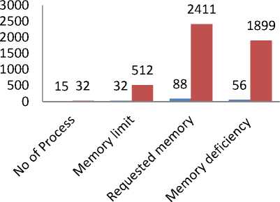
Category A: Table 2 below shows a computer system with a total of 15 created processes, all with their system information in Figures. The computer memory can accommodate capacity of 32mb.
Category B: Table 3 below shows system information of a total of 32 data/processes in Figs. The memory capacity of this system is 512mb.
From Table 2, there are a total of 15 processes and that of Table 3 has 32 processes. Taken the system information each process carries, if all processes are allowed to load as soon as created, from Table 2, the computer system will require total memory capacity of 88mb exceeding the main memory capacity of 32mb. Table 3 will demand an arbitrary overall memory space of 2411mb from a System with capacity limit 512mb. Therefore, from Table 2, an additional memory of 56mb needs to be created and that of Table 3 is1899mb.
Therefore, it is infeasible to allow all the process to run without running into low memory or system crushes. A summary is shown in Fig. 1
Table 2. Data values of Category A
|
Processes No |
data size/mb |
Number of times data is accessed |
|
1 |
6 |
6 |
|
2 |
4 |
5 |
|
3 |
8 |
8 |
|
4 |
6 |
2 |
|
5 |
6 |
9 |
|
6 |
7 |
4 |
|
7 |
5 |
7 |
|
8 |
7 |
9 |
|
9 |
3 |
6 |
|
10 |
10 |
2 |
|
11 |
3 |
9 |
|
12 |
6 |
10 |
|
13 |
9 |
9 |
|
14 |
5 |
8 |
|
15 |
3 |
6 |
|
Total: 88 |
Table 3. Data values of Category B
|
Processes No |
Memory data size/mb |
Number of times data is accessed |
|
1 |
25 |
6 |
|
2 |
52 |
5 |
|
3 |
100 |
7 |
|
4 |
86 |
9 |
|
5 |
36 |
5 |
|
6 |
76 |
3 |
|
7 |
12 |
4 |
|
8 |
56 |
7 |
|
9 |
128 |
7 |
|
10 |
96 |
7 |
|
11 |
160 |
8 |
|
12 |
120 |
3 |
|
13 |
82 |
2 |
|
14 |
68 |
4 |
|
15 |
92 |
6 |
|
16 |
48 |
5 |
|
17 |
128 |
4 |
|
18 |
160 |
8 |
|
19 |
24 |
6 |
|
20 |
64 |
2 |
|
21 |
96 |
1 |
|
22 |
124 |
3 |
|
23 |
65 |
2 |
|
24 |
12 |
3 |
|
25 |
45 |
7 |
|
26 |
56 |
6 |
|
27 |
86 |
7 |
|
28 |
82 |
3 |
|
29 |
98 |
7 |
|
30 |
134 |
8 |
|
31 |
142 |
4 |
|
32 |
200 |
5 |
|
Total: 2753 |
■ Table 4.1 ■ Table 4.2
Fig.1. Memory demand of Table 1 and Table 2
Strategy one allows data/process to be loaded according to data size picking data with smallest sizes first until the system capacity is reached. From Table 2, processes 1, 2, 4, 7, 9, 11 satisfy the condition over the other processes and therefore by precedence it will be given concern. Together, this six (6) data/process will require 28mb space, with 4mb free. From Table 4.2, processes 1, 2, 5, 7, 8, 16, 19, 20, 23, 24, 25, and 26, a throughput of 12 data/processes satisfy the condition with a total request memory of 495mb, 17mb space left unused.
Table 4 compares the optimal data from Table 2 of Load data into memory by size Strategy and the Dynamic Programming approach.
Table 4. Comparism of Optimal Data of Table 2
|
Load data into memory by size (Strategy 1) |
Dynamic Programming Approach |
||
|
ProcessNo |
data size/mb |
ProcessNo |
Data size/mb |
|
1 |
6 |
5 |
6 |
|
2 |
4 |
7 |
5 |
|
4 |
6 |
9 |
3 |
|
7 |
5 |
11 |
3 |
|
9 |
3 |
12 |
6 |
|
11 |
3 |
14 |
5 |
|
15 |
3 |
||
Table 5. Comparism of Optimal Data of Table 3
|
Load data into memory by size(Strategy 1) |
Dynamic Programming Approach |
||
|
Processes No |
data size/mb |
Processes No |
Data size/mb |
|
1 |
25 |
1 |
25 |
|
2 |
52 |
2 |
52 |
|
5 |
36 |
3 |
100 |
|
7 |
12 |
4 |
86 |
|
8 |
56 |
5 |
36 |
|
16 |
48 |
7 |
12 |
|
19 |
24 |
8 |
56 |
|
20 |
64 |
19 |
24 |
|
23 |
65 |
24 |
12 |
|
24 |
12 |
25 |
45 |
|
25 |
45 |
26 |
56 |
|
26 |
56 |
||
Table 5 compares the optimal data from Table 3 of
Load data into memory by size Strategy and the Dynamic Programming approach.
Table 6. Memory utilisation Analysis of Table 2
|
Specification |
(Strategy 1) |
Dynamic Programming Approach |
|
System throughput |
6 |
7 |
|
Memory acquired |
28 |
31 |
|
Used memory |
4 |
1 |
System Memory Used throughput acquired memory
-
■ (Strategy 1)
-
■ Dynamic Programming Approach
-
Fig.2. Memory utilisation of Table 6
Table 6 illustrate the analysis of Memory utilisation of
Table 2 whereas Table 7 illustrate the analysis of
Memory utilisation of Table 3
Table 7. Memory Utilisation Analysis of Table 3
|
Specification |
(Strategy 1) |
Dynamic Programming Approach |
|
System throughput |
12 |
11 |
|
Memory acquired |
495 |
504 |
|
Used memory |
17 |
8 |
|
600 |
495 504 |
|
|
500 |
||
|
400 |
||
|
300 |
||
|
200 |
||
|
100 0 |
12 11 |
17 8 |
System Memory Used memory throughput acquired
-
■ (Strategy 1)
-
■ Dynamic Programming Approach
-
Fig.3. Memory utilisation of Table 7
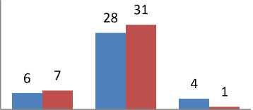
Strategy two allows data/process to be selected according to the number of times data is access or the data access times until the system capacity is reached. Passing the data in Table 2 through this heuristic strategy, processes 5, 8, 11, 12, and 13 satisfy the condition due to its higher access times. A throughput of 5, it requires
Table 8. Comparism of Optimal Data of Table 2
|
Load data into memory by number of accesses (Strategy 2) |
Dynamic Programming Approach |
||
|
Processes No |
Number of times data is accessed |
Processes No |
Number of times data is accessed |
|
5 |
9 |
5 |
9 |
|
8 |
9 |
7 |
7 |
|
11 |
9 |
9 |
6 |
|
12 |
10 |
11 |
9 |
|
13 |
9 |
12 |
10 |
|
14 |
8 |
||
|
15 |
6 |
||
31mb space to manage this processes.
Processes 4, 11, and 18 giving a throughput of 3 from Table 3 satisfy the condition of heuristic strategy two. The processes will require 406mb to allow the three most frequently accessed data to run in memory holding the remaining data/process in queue. This will leave 106mb free space in memory unutilized.
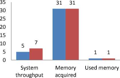
Using the Dynamic programming approach for solving Table 2 as already illustrated in Fig 2, a throughput of 7, Processes 5, 7, 9, 11, 12, 14, and 15 is loaded into memory for CPU scheduling. With Table 3, Processes 1, 2, 3, 4, 5, 7, 8, 19, 24, 25, 26 totalling a throughput of 11 is loaded for memory allocation since their memory utilisation requirement is 8mb less than the 512mb memory capacity of the computer system. This is illustrated in Fig 3.
Table 8 compares the optimal data from Table 2 of Load data into memory by number of accesses Strategy and the Dynamic Programming approach.
Table 10: Memory utilisation of Table 2
|
Specification |
(Strategy 2) |
Dynamic Programming Approach |
|
System throughput |
5 |
7 |
|
Memory acquired |
31 |
31 |
|
Used memory |
1 |
1 |
-
■ (Strategy 2)
-
■ Dynamic Programming Approach
Fig.4. Memory utilisation of Table 10
Table 11. Memory utilisation of Table 3
|
Specification |
(Strategy 2) |
Dynamic Programming Approach |
|
System throughput |
3 |
11 |
|
Memory acquired |
406 |
504 |
|
Used memory |
106 |
8 |
Table 9 compares the optimal data from Table 3 of Load data into memory by number of accesses Strategy and the Dynamic Programming approach.
Table 9. Comparism of Optimal Data of Table 3
|
Load data into memory by number of accesses (Strategy 2) |
Dynamic Programming Approach |
||
|
Processes No |
Number of times data is accessed |
Processes No |
Number of times data is accessed |
|
4 |
9 |
1 |
6 |
|
11 |
8 |
2 |
5 |
|
18 |
8 |
3 |
7 |
|
4 |
9 |
||
|
5 |
5 |
||
|
7 |
4 |
||
|
8 |
7 |
||
|
19 |
6 |
||
|
24 |
3 |
||
|
25 |
7 |
||
|
26 |
6 |
||
|
600 |
504 |
||
|
500 |
406 |
||
|
400 |
|||
|
300 |
|||
|
200 |
106 |
||
|
100 0 |
3 11 |
■ |
8 |
|
System |
Memory |
Used |
|
|
throughput |
acquired |
memory |
|
|
■ (Strategy 2) |
|||
|
■ Dynamic Programming Approach |
|||
Fig.5. Memory utilisation of Table 11
Table 10 illustrate the analysis of Memory utilisation of Table 2 for strategy two
Comparing the Dynamic programming approach to other existing strategies employed by computer programmers and system developers for optimising memory, the Dynamic programming approach tends to out-perform most of them.
The Dynamic programming approach tends to pick data/process that can enhance efficient utilisation of memory. It also picks as many processes as possible provided their data sizes do not exceed the system capacity. from Table 6 even though loading data into memory by size strategy (Strategy one) allowed system throughput of 6, it left an unused memory space of 4mb compared to the Dynamic approach of allowing 7 process, and an efficient memory utilisation of 31mb, illustrating that there is optimal utilisation of memory. Same can be made of Table 7 with strategy 1 picking more data/process than the Dynamic approach, it left more unutilized space than the Dynamic approach which may lead to memory leakage. The strategy of loading data into memory by size strategy tends to favour only process/data with smaller data size but data with larger data size takes a long time to be given space thereby increasing the allocation time of such data irrespective of the higher system priority or access frequency that a data/process may have.
The second strategy although can be used to Optimize memory, it also failed to perform better compared to the proposed approach. From Table 10, although the memory requirement of selected processes of Table 2 for Load data into memory by number of accesses strategy (strategy 2) equals the Dynamic programming approach, the system throughput of the heuristic strategy two falls short of 2 more processes compared to the Dynamic programming approach which allow 7 processes to load at time. In Table 11 the Dynamic programming approach achieves 8 more processes than heuristic strategy two. With only 3 system throughput, strategy two require 406mb memory spaces to allow the most frequently used process to run leaving behind 106mb memory unutilized. The Dynamic programming approach, with 11 system throughput, made an effective utilisation of memory. It required 504mb memory leaving 8mb space free. At this point it can be deduced that The Load data into memory by number of accesses strategy may sometimes not make use of efficient use of memory and may lead to memory loses and leakages
Additionally, the Load data into memory by number of accesses strategy take a longer time for a fresh new data to be loaded into memory space since it favours data/process with a higher number/time accessed otherwise such process/data is held in queue. Therefore, newly created process which probably may need little space to load will have to wait a long while to execute.
V. Conclusion
In this paper, we propose a partial enumeration technique based on an exact enumeration algorithm like the dynamic programming for effective utilisation and optimization of memory. The problem identified is one that has a single linear constraint, a linear objective function which sums the values of data/process in memory, and the added restriction that each data/process should be in memory or not. The Dynamic programming approach proved to quickly find an optimal solution or a near optimal solution in some situations where exact solution is not possible as opposed to a heuristic that may or may not find a good solution.
From the paper, it is shown that the Dynamic programming algorithm is more efficient and yield better result than other existing heuristic algorithm. Dynamic Programming algorithm is easy to implement since no sorting is necessary, saving the corresponding sorting time. Additionally, the time complexity taken to solve the Dynamic programming is 0(n*W) compared to the 0/1 knapsack algorithm running time of O(2^n). Taken that n is the number of items and W is the Capacity limit.
References Optimizing Memory using Knapsack Algorithm
- Gil-Lafuente, A., de-Paula, L., Merig-Lindahl, J., M., Silva-Marins, F., and de Azevedo-Ritto, A. (2013). Decision Making Systems in Business Administration: Proceedings of the MS'12 International Conference. World Scientific Publishing Co., Inc. Retrieved from http://dl.acm.org/citation.cfm?id=2509785
- Silberschatz, A., and Peterson, J. (1989). Operating System Concepts. Addison-Wesley, Reading.
- Chen G., Chern M., and Jang J. Pipeline architectures for dynamic programming algorithms. Parallel Computing, 1(13):111 – 117, 1990.
- Coquand,T., Dybjer, P., Nordström, B., and Smith, J. (1999). Types for Proofs and Programs, International Workshop TYPES'99, Lökeberg, Sweden, Available from: Selected Papers. Lecture Notes in Computer Science 1956, Springer 2000, ISBN 3-540-41517-3.
- Pisinger, D. (1994). Core problems in knapsack algorithms. Operations Research 47, 570-575.
- Kellerer, H., Pferschy, U., Pisinger, D. (2004). Knapsack Problems. Springer, Berlin Heidelberg.
- Cáceres E. N., and Nishibe, C. (2005). 0-1 Knapsack Problem: BSP/CGM Algorithm and Implementation. IASTED PDCS: 331-335.
- Robert M, & Thompson, K (1978). Password Security: A Case History. Bell Laboratories, K8.
- Chu P.C and Beasley J. E. (1998), A genetic algorithm for multidimensional knapsack problem. Journal Heuristics. 4:63-68.
- Oppong, O. E. (2009). Optimal resource Allocation Using Knapsack Problems: A case Study of Television Advertisements at GTV. Master's degree paper, KNUST.
- Kalai, R. and Vanderpooten, D. (2006). Lexicographic a-Robust Knapsack Problem http://ieeexplore.ieee.org/xpl/freeabs
- Benisch, M., Andrews, J., Bangerter, D., Kirchner, T., Tsai, B. and Sadeh, N. (2005). CMieux analysis and instrumentation toolkit for TAC SCM. Technical Report CMU-ISRI-05-127, School of Computer Science, Carnegie Mellon University.
- Shang, R., Ma, W. and Zhang, W (2006). Immune Clonal MO Algorithm for 0/1 Knapsack Problems. Lecture Notes in Computer Science, 2006, Volume 4221/2006, 870-878.
- Kosuch, S. and Lisser, A. (2009). On two-stage stochastic knapsack problems. Discrete Applied Mathematics Volume 159, Issue 16.
- Florios, K. et. al. (2009). Solving multi objective multi constraint knapsack problem using Mathematical programming and evolutionary algorithm. European Journal of Operational Research 105(1): 158-17.
- Horowitz, E. and Sahni, S. (1972). Computing partitions with applications to the Knapsack Problem. Journal of ACM, 21, 277-292.
- Nauss, R,. M. (1976). An Efficient Algorithm for the 0-1 Knapsack Problem. Management Science, 23, 27-31.
- Martello, S., Pisinger, D. and Paolo, T. (2000). New trends in exact algorithms for the 0 – 1 knapsack problem. http: // citeseerx.istpsu/viewdoc/download?doi10.1.11.89068rep=rep| type=ps
- Silva et.al (2008). Core problem in bi criteria 0-1 knapsack problems. Retrieved from: www.sciencedirect.com
- Yamada, T, Futakawa, M., and Kataoka, S. (1998). Some exact algorithms for the knapsack sharing problem. www.sciencedirect.com
- Lin and Wei (2008). Solving the knapsack problem with imprecise weight coefficients using Genetic algorithm. www.sciencedirect.com
- Bortfeldt A, Gehring H. (2001). A hybrid genetic algorithm for the container loading problem [J]. European Journal of Operational Research, 2001, 131(1):143-161.
- Simoes, A, and Costa, E. (2001). Using Genetic Algorithm with Asexual Transposition. Proceedings of the genetic and evolutional computation conference (pp 323-330).
- Babaioff, M. et al (2007). Matroids, secretary problems, and online mechanisms. Proceedings of the eighteenth annual ACM-SIAM symposium on Discrete algorithms. Pages 434-443
- Hanafi, S. and Freville, A. (1998), An efficient tabu search approach for the 0-1 multidimensional knapsack problem. http://www.sciencedirect.com
