Особенности метода восстановления Ne на Иркутском радаре некогерентного рассеяния

Despite the fact that the method of incoherent scattering (IS) has been existing for more than fifty years, it still remains the most informative. It allows us to restore ionospheric parameters such as the electron density N e , ion T i and electron T e temperatures, and several other characteristics in a wide range of heights (50–1000 km) from high-frequency electromagnetic wave (frequency higher than the plasma one) scattering by weak fluctuations of plasma permittivity [Dougherty, Farley, 1961] .

The practical implementation of the task of restoring the ionospheric parameters from data obtained by the IS method is extremely difficult. We should take into account that the scattered signal itself is very weak. The signal-to-noise ratio is considerably less than unity since only a small portion of wave energy is scattered by minor permittivity fluctuations. Hence, to detect a backscattered signal there is a need for instruments with both considerable energy potential and high sensitivity. This requires the use of the most advanced achievements in electronics and related disciplines. In addition, plasma parameters are restored using procedures belonging to the class of inverse problems [Tarantola, 1987] .

Two values serve as experimental data in ionospheric observations: the height dependence of signal power to determine Ne and the frequency distribution of energy density that allows us to estimate ion and electron temperatures and plasma ion composition from the spectrum shape. The drift velocity of plasma as a whole along the line of sight can be inferred by the frequency shift of the spectrum due to the Doppler effect. A connecting link is a radar equation [Suni et al., 1989], which also takes into account parameters of the transceiver path of a radar and the form of a probe signal in use.

Because the models describing, say, the spectrum of fluctuations [Akhiezer et al., 1974] are multiparameter and nonlinear, procedures for searching parameters become incorrect; and solutions, unstable. Therefore, the methods of analyzing IS signals and the instruments continue being developed [Holt et al., 1992; Vierinen et al., 2007] in order to meet the increasing requirements for precision and elimination of ambiguity in restoring vertical profiles of ionospheric parameters.

To meet the modern requirements for ionospheric measurements, Russia’s unique IS radar — the Irkutsk Incoherent Scatter Radar (IISR) — has been modernized [Zherebtsov et al., 2002; Potekhin et al., 2008; Potekhin et al., 2009] . The IISR antenna emits and receives strictly linearly polarized signals, which distinguishes IISR from all existing radars. On the one hand, this requires the development of new IS signal processing methods; on the other hand, this allows us to recover absolute values of N e from signal fading caused by the Faraday effect, i.e. rotation of the wave polarization plane.

The modernization of the IISR hardware and software complex has opened up new possibilities for diagnostics of the ionosphere by the IS method. At the same time, a new technique for restoring ionospheric plasma parameters has begun to be devised in order to eliminate disadvantages of the previously developed algorithm [Shpynev, 2000; Shpynev, 2004] . According to [Shpynev, 2000] , we can conclude that the disadvantages of the old algorithm include: deconvolution of the IS signal power profile with the probe signal; multiplication of Faraday variations in the signal power profile by squared distance determining a quadratic increase in the noise level; unrealistic variations in the recovered N e near the minimum power profile even for

This is an open access article under the CC BY-NC-ND license small changes of noise in this region; phase differentiation. These problems cause instability in determining ionospheric parameters. This is most pronounced during solar minimum due to a low signal-to-noise ratio and a minimum number of Faraday variations in the signal power profile. Moreover, the old algorithm requires manual processing. To overcome these disadvantages and improve the accuracy of restoration of the ionospheric plasma parameters, we have developed a new method that does not require manual processing.

OVERVIEW OF METHODSFOR RESTORING THE ELECTRONDENSITY PROFILE

where P is the radiated power; G 0 is the antenna gain; λ is the radiation wavelength; r is the height along the radar beam; а(т) is the probe pulse shape; F tr (s, y), F r (s, γ) is the function modulus describing the field pattern shape during transmission and reception; Q (τ) is the noise of both natural and instrumental origin; Ω ( r ) is the rotation angle of the wave polarization plane proportional to the total electron content along the propagation path [Evans, 1969; Shpynev, 2004] :

e ³       r

^Q ( Г ) = ^---— f N e ( z ) B ( z ) cos a dz ,         (2)

^{2 e} 0 m e ® 0 c 0

According to the incoherent scattering theory, there are three basic ways to restore the vertical profile of N e ( r ): 1) by measuring the total power of a received signal; 2) by measuring the Faraday rotation profile; 3) by measuring the plasma line.

The first way is the easiest to determine the height variation in N e . In this case, in the experiment in the transmission and reception we use a circularly polarized electromagnetic wave, and the power profile becomes proportional to N e . The absolute values of N e are recovered by normalizing to the maximum electron density, measured, for example, by a nearby ionosonde. The correction for the ratio of electron and ion temperatures is made from correlation measurements. Due to the simplicity of such measurements, most IS radars use a circularly polarized signal and/or a circularly polarized receiving antenna, thus eliminating the Faraday effect.

Nevertheless, the Faraday effect is utilized in recovering the N e vertical profile and in radars whose antennas are circularly polarized, such as ISR in Kharkov [Tkachev, Rozumenko, 1972] . Since this radar cannot completely eliminate the mutual influence of orthogonal components of a received signal, a special method for recovering the vertical profile of N e has been developed [Grigorenko, 1979] , which is based on the analysis of extreme points of the power profile. The method works well at F2-layer heights when the electron density is high in the daytime. At a low electron density there is generally lack of the extreme points for N e reconstruction with appropriate height resolution.

IISR emits and receives only a linearly polarized electromagnetic wave, thus considerably complicating the recovery of the height variation in N e . Propagating in the ionospheric plasma located in the external geomagnetic field, a linearly polarized electromagnetic wave breaks down to ordinary and extraordinary waves. Because of the difference between their phase velocities, the Faraday rotation of the total signal polarization plane occurs [Ginsburg, 1967] , resulting in the dependence of the electromagnetic wave polarization vector on the rotation angle in the radar equation describing the received IS signal power for the linearly polarized receiving antenna [Bernhardt, 2000] :

where ω 0 is the carrier frequency; e is the electron charge; ε 0 is the permittivity; m e is the electron mass; c is the velocity of light; z is the height; B ( z ) is the geomagnetic field.

The method of restoring the vertical profile of N e absolute values from the signal with Faraday variations in its power profile is described in detail in [Shpynev, 2000; Shpynev, 2004] . This method has, however, both an advantage of being able to recover small-scale irregularities and disadvantages described above. Particularly noteworthy is the considerable sensitivity of the algorithm to the noise level, which consists in unstable determination of ionospheric plasma parameters. This was the major cause of the serious distortions of the restored vertical electron density profiles during solar minimum. Let us take a brief look at this method.

As can be seen from Equation (1), we should first solve the equation of convolution relative to |a ( t- 2 c/c )|². This procedure is the deconvolution, its task is to eliminate the influence of the probe signal, which leads to the fact that the minimum Faraday variations in the signal power profile blur and do not decrease to the noise level (see Figure 1). The deconvolution problem belongs to the class of incorrect problems requiring the use of special regularizing algorithms, and its solution exhibits instability, which greatly increases in noise.

The deconvolution is described in detail in [Voronov, Shpynev, 1998] . To overcome the instability, primary emphasis was placed on such a property of the probe pulse as its squareness, and the problem was solved for an almost rectangular kernel. This deconvolution algorithm is inapplicable to complex signals (e.g., phaseshift). According to this algorithm, Equation (1) is transformed into the following expression:

P ( c ) = n c 2 A

N _; ⁽ Г ^)cos 2 ( Q ⁽ Г ) ) + Q ₍ r ) c ² ( 1 + T_e(r )/ T(r ) )

PG2V 2 ,

P(t) = /0 A3 e f Ftr (e, YF (e, Y)cossdedyx (4л)

N ₌ ( Г ) ^cos 2 ( Q ( Г ) ) ^{X f}    1 + T e ( Г ) T ( Г )

а

dr

where A is the factor depending on specifications of the antenna system.

It is Equation (3) that is used to solve the problem of restoring the N e ( r ) profile. This equation has a double dependence on N e ( r ). On the one hand, the electron density enters into this equation as a factor, on the other hand, it is included in the expression for phase Ω ( r ) and according to Expression (2) it is a phase derivative:

Q ^(t) ,

N . (,) = 1 d ^ < r >, Y dc

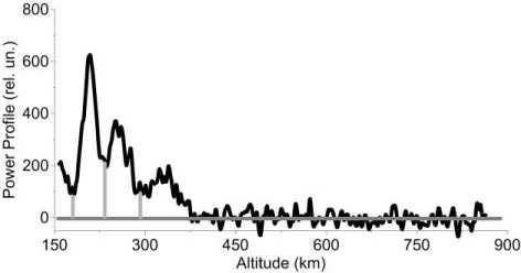
Figure 1. Effect of probe pulse where

• e ³ B cos a

• Y= .    2_2 .

2 ⁸ о m e to o c

Substituting (4) in (3), multiplying both sides by r ² ( 1 + T_e ( r)/ T ( r ) ) and, integrating, we get

r

• —2 J P ( r ) r² ( 1 + T e ( r ) / T i ( r ) ) dr +

^{П Г} е A 0

r

+ -2- J Q(r)r2 (1 + Te (r) / T (r)) dr =         (5)

ⁿ r e A 0

sin ( 2 Q ( r ) )

= Q( r) +----^ + c.

Expression (5) shows the main factors that cause the instability of the algorithm. The first one suggests that the multiplication of noise power by squared distance leads to a quadratic increase in the noise level, which is significant at high altitudes, where the signal-to-noise ratio is reduced significantly. The second implies the presence of a noise in power profile minima, small variations of which cause unrealistic N e ( r ) variations, which requires manual setting of positions of all the minima and special measures in their vicinity for phase calculations. When restoring N e ( r ), as seen from Expression (4), we should differentiate the obtained phase. This operation leads to significant changes in the obtained values in the case of even slight phase variations.

The above factors preclude the development of a fully automated procedure for recovering the altitudetemporal behavior of N e . Below is a method of automated processing of IISR data, which takes into account features of the radar (linear polarization).

STRUCTUREOF THE NEW METHOD

We can significantly increase the stability of the algorithm of restoring the vertical electron density profile, using parametric models. This method meets the modern requirements for measurements and has been widely used recently. It involves determining ionospheric plasma parameters throughout the height range of interest [Holt et al., 1992; Lehtinen, Huuskonen, 1996] .

In this case, the restoration of the parameters in general involves several steps. The first step is to choose a parametric model describing the behavior of an object under study. The second step is to determine the method of searching for parameters of the model and regularizing algorithms. The determination methods generally reduce to a fitting procedure (fitting of the model function to experimental data) and are standard. The final step is to determine the parameters with which the selected model can best describe experimental data.

In the case of IISR, when specifying a parametric model of the N e ( r ) profile, we can eliminate the Ω( r ) phase differentiation. We can also remove the quadratic increase in the noise level when multiply it by the squared distance due to the absence of the latter in the model. The application of the model specifying the entire height variation in N e ( r ) allows us to avoid unrealistic variations in N e for small changes of noise, which occur in power profile minima when N e ( r ) is calculated at each point. Instead of the deconvolution procedure, the standard procedure of convolution of the model power profile and the ambiguity function of the signal used in the experiment is applied to the probe pulse shape.

Before describing the method in detail, let us briefly run through approximations and features of IISR operation used for its development. The technical and software upgrade of IISR enabled us to use complex signals such as those with phase modulation for ionospheric measurements on a regular basis. Signals of this type make it possible to find a compromise between height resolution and energy of the emitted signal. The main type of phase manipulation in the experiments is a Barker code. It provides information on medium parameters with a spatial resolution of few kilometers (1.5 to 6 km at a pulse length of ~200 µs and Barker codes 5–13). The spatial resolution achieved due to the use of signals with phase manipulation allowed us to eliminate the deconvolution in a first approximation. The ratio of electron temperature to ion temperature is assumed to be equal to unity throughout the height range. Using these approximations, we can considerably simplify radar equation (1):

N e ⁽ r ^)cOs² ( Q ⁽ r ) )

P ⁽ r ) = n r, A ----------2-^------'-.          (6)

r

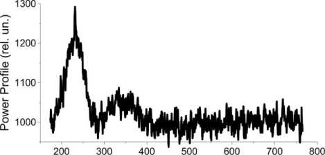
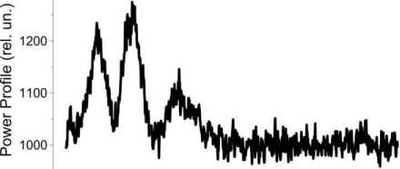
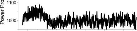
As mentioned above, the altitude-temporal behavior of the electron density is recovered from the experimentally measured scattered signal power. Directly in the experiment a two-dimensional sequence is observed — a discrete set of N readings with a given sample spacing describing the altitude-temporal behavior of the squared sum of IS signal and noise. Such an altitude sequence of N readings is one implementation. A low signal-to-noise ratio requires the use of statistical methods [Bard, 1974; Dennis, Schnabel, 1983] to describe IS experimental data. In our work, we assume that the noise in the experiment is normally distributed. Then, using the central-limit theorem, we can give probabilistic estimates of the variance and mean power of a scattered signal by integrating independent realizations of the received signal in the time interval in which the ionosphere can be considered constant. In practice, to collect sufficient statistics we should average at least 3000 independent realizations (which at a pulse repetition frequency of 24.4 Hz is 4 min), where- as in most experiments the averaging time is 15 min. Figure 2 gives examples of vertical profiles of IS signal power for the conditions corresponding to the dayside, evening, and nightside ionosphere in summer at low solar activity.

The lower boundary of the ionosphere is considered to be a height of ~50 km, but for IISR the terrain imposes restrictions on the minimum height at which we can receive an IS signal [Potekhin et al., 2008; Potekhin et al., 2009] . Reflections from mountains in a height range to ~160 km have an amplitude much higher than that of scattered signal, thus precluding the identification of IS signal from heights below 160 km. For this reason, hereinafter we use a single-layer model of electron density profile for the F2-layer height range. Methods of noise subtraction from terrain objects are currently being developed for IISR [Tashlykov et al., 2019] , which implies a complication of the electron density profile model in use.

The geomagnetic field in [Shpynev, 2004] is considered constant, but models show its height dependence for a range 100–1000 km (a twofold maximum change). In our calculations, the height dependence of the geomagnetic field is set by the IGRF model [Tsyganenko, 2002a, b] .

As a method for determining optimal parameters of the

Altitude (km)

200     300     400     500     600     700     800

Altitude (km) 1300

05 1200

Ф

200     300     400     500     600     700     800

Altitude (km)

Figure 2. Vertical profiles of IS signal power (top to bottom) for conditions of the evening, dayside, and nightside ionosphere in summer at low solar activity model, at which it most reliably represents experimental data, we utilize the method of least mean squares:

3 = S ( Y ⁽ K ) - ^P0 ⁽ K , x ) ) ² ^ ^min-               ⁽⁷⁾

Here Y e ( r i ) is experimental data; P 0 is the parametric model; r i is the distance along the radar beam, the vector x contains the model parameters to be determined. It is, however, necessary to take into account the receive path gain and the noise level regardless of the model chosen. Both these values may be time dependent, and their account is equivalent to introducing two additional parameters into the model:

5 = s ( Y _exp( r i ) - AP₀(r , x ) - C ) ² ^ min,         (8)

where A is the gain; C is the noise level.

The model parameters ( A and C ) linearly entering Expression (8) can be determined by solving the system of linear equations, which can be obtained from the condition of equality of partial derivatives with respect to these parameters to zero. Nonlinear parameters are found either by searching or by gradient methods. One of these parameters is the initial phase incursion, caused by IISR’s inability to measure the signal power below 160 km.

Let us begin the detailed description of the method with a priori information to determine the initial phase incursion as a function of time. This information is needed to automate the method. Radar equation (6) includes an integral of the electron density; and a loss of information on the behavior of the useful signal power at heights to 160 km due to the restriction on the minimum receiving height makes it impossible to determine the model IS-signal profile. Let us introduce the parameter Ω 0 — integral of the electron density in the 50–160 km height range:

r

Q ( r ) = y j N ( z ) B ( z ) cos a dz =

r

= Q_o ( r ) + y j N _e ( z ) B ( z ) cos a dz ,

where r 0 is the height (in our case, ~160 km) above which a scattered signal from ionospheric plasma begins to be detected.

As can be seen, the residual nonlinearly depends on Ω 0 , and the determination of Ω 0 is challenging since we have to ensure stability and uniqueness of the solution. In this paper, we use the direct searching method for finding Ω 0 , therefore we should first determine the acceptance region for this parameter. According to radar equation (6), the power of the signal received with IISR depends on the rotation angle of the polarization plane as a squared cosine. The cosine vanishes when the argument is π/2+π n , with the first zero cos(π/2) corresponding to the first signal power minimum. Let us use the experimental data to trace changes in heights of the first signal power minimum and maximum depending on the time of day and season.

Figure 3 shows altitude-temporal variations of IS signal power on January 01, 2014. We can see that at 0–1 UT (dawn local time) there is the first maximum of Faraday

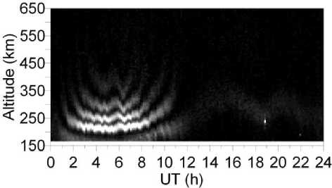
Figure 3 . Behavior of the altitude-temporal profile of Faraday variations in signal power on January 01, 2014 (LT=UT+7)

variations in the signal power profile at ~250 km followed by the first minimum at ~350 km. Between 02 and 07 UT (day conditions), the height of the first maximum is below 160 km, whereas the height of the first minimum is above 160 km. Then (from 08 UT), the first maximum and minimum again begin to rise, reaching the greatest heights in the nighttime (14–22 UT). At dawn (after 22 UT), these structures repeat the behavior.

Figure 4 shows altitude-temporal variations in power of the signal modulated by the Faraday effect, measured in winter, spring, summer, and fall, and diurnal variations of the cosine of the solar zenith angle corresponding to these seasons (red curve) [Daffet Smith 1982]. To formalize the calculation algorithm, it is convenient to associate variations of the first signal power maximum and minimum with diurnal variations of the solar zenith angle in different seasons. The height region of localization of the first signal power minimum (the first zero, hence Ω0) is seen to depend largely on the time of day and to be essentially independent of season. To fit the heights of the first zero to the zenith angle, we take four times of day: night, dawn, day, dusk. Day and night are the times of day separated by dawn and dusk. Dusk is believed to be the time when the first maximum rises. To it correspond values of the cosine of the solar zenith angle in a range from 0.15 to –0.15. In turn, dawn is the time of day when the first maximum goes down, and the cosine of the solar zenith angle ranges from –0.15 to 0.15. Vertical lines in Figure 4 indicate transitions from day to dusk and from dawn to day (red lines), from dusk to night and from night to dawn (green lines). Ranges of height variations in the first zero for each of the time of day, determined from large statistics, are listed in the Table.

Figure 4 shows that the height of the first signal power minimum never becomes less than the minimum accessible for observation (~160 km). A further analysis of a wide array of both new and old experimental data has revealed that the first signal power minimum repeats the described behavior for different seasons and solar activity levels. Thus, Ω 0 (9) may vary from 0 to π/2 (when searching, just in case, we use the range [0, π/2+π/10]). In multiparameter optimization problems, it is important to ensure stability of the solution.

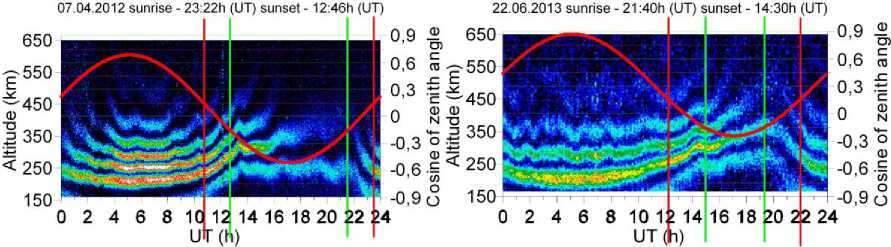
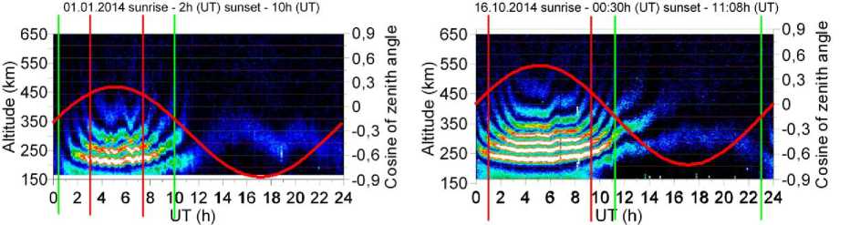
Figure 4 . Altitude-temporal behavior of a received signal modulated by the Faraday effect for winter, spring, summer, fall periods (LT=UT+7): diurnal variation in the cosine of the solar zenith angle (red curve); vertical red lines mark transitions from day to dawn and from dawn to day; green lines, from dusk to night and from night to dawn

Height range of the first minimum of Faraday variations in signal power profile depending on the time of day

	day	dusk	night	dawn
Height range, km	160–240	190–300	250–450	230–400

This statistics is used for regularization. When searching Ω 0 values, we consider only those Ω 0 for which the corresponding first zero height is in the ranges listed in the Table. The use of such regularization enabled us to develop a fully automated algorithm.

Let us now consider a practical implementation of the method. As a model profile we use a combination of two Chapman layers. The Chapman layer is the most common approximation, which also is the main in restoring the vertical profile of N e above the ionization maximum in an ionosonde. Its advantages include smoothness, which is important for solving nonlinear problems classed as inverse, but this model cannot describe small-scale variations. The analytical expression for the Chapman layer in the case of different thicknesses above and below the peak height has the form

The algorithm works as follows. For all possible variables of N m F2, h m F2, H B , and H T , a set of N e model profiles is constructed. Then, for each N e profile (the magnetic field behavior with height is preset) we calculate the profile of the rotation angle of the electromagnetic wave polarization plane from the formula

^Q ( r) = -- —N m F2 x

2 E o m e to_Q c

r xj exp (1 - x - exp(-x))B(z)cos adz.

r ₀

N e ( z ) = N m F2 X

x =

x exp ( 1 - x

exp( - x ) ) <

z — h _mF2 H B

if z <  h _mF2

x=

z — h _mF2

H _T

if z >  h m F2,

where z is the height; N m F2 is the maximum electron density; h m F2 is the peak height; H B and H T is the thickness of the inner (below h m F2) and outer (above h m F2) ionosphere respectively. These parameters, along with the phase Ω 0 , are unknown and should be determined. Figure 5 shows the model electron density profile with its four parameters.

For these parameters we should also define the range of their variation. Thus, the maximum electron density ( N m F2) varies within [0.5÷32]·10⁵ cm^–3 in increments of 0.5·10⁵ cm^–3; the height of maximum electron density ( h m F2) varies from 200 to 450 km in increments of 5 km; the range of variation of the lower and upper half-thickness of the F2 layer is from 20 to 160 km in increments of 5 km. If necessary, the increments and ranges can be varied.

The next step is to compute a similar set of profiles of signal fading, caused by the Faraday effect, from the calculated angle. Then, at the input of the model we specify an experimental fading profile and compare each model fading profile, obtained taking into account all distorting factors, with the experimental profile. The comparison is made until the best model profile with a minimum of residual and regularizing conditions being met is found.

After determining an appropriate signal fading profile, we automatically define all necessary parameters of its corresponding vertical profile of N e ( r ).

Figure 6 depicts an experimental profile of signal fading, which is an input parameter, and the profile of signal fading recovered from a model profile of N e ( r ), as well as the model profile of N e ( r ). Circles with numbers mark signal fading.

We can see that the number of parameters to be recovered is equal to five. The inverse problem itself is known to be extremely unstable, and with a large number of parameters the instability rises exponentially.

For stabilizing it, we used the maximum amount of a priori information. For phase, a priori information has been described above. The peak height and maximum electron density are given by the form of signal fading caused by the period of minima and their location. At night, when the Faraday effect, in particular by the repetition number of variations is small (the problem of one hump), information on the phase plays a significant role. To provide

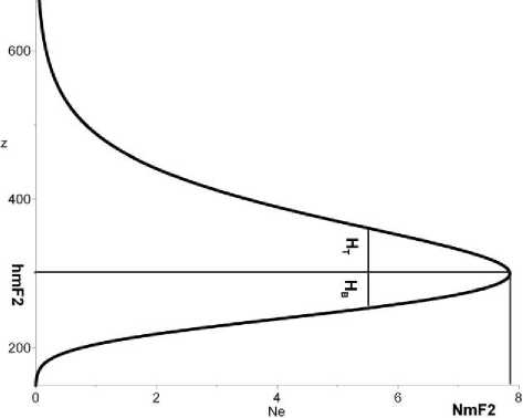
Figure 5 . Vertical electron density profile described by the Chapman layer of different thickness above and below the peak height

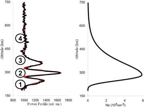
Figure 6 . Profiles of signal fading caused by the Faraday effect (left): observed experimentally (black curve) and restored (red curve) from the model N e profile; model N e ( r ) profile (right)

even greater stability, we can specify the range of variations in A or C . It is easier to make for C . In this case, it suffices to determine the noise intensity from the end of the scanning window and to specify a deviation from this value. It is much more difficult to control the parameter A because we must know how characteristics of the antenna system change with time.

The computational complexity of the algorithm is quite high, therefore we have taken steps to optimize it. As mentioned above, the height dependence of the geomagnetic field is specified by the IGRF model [Tsyganenko, 2002a, b] . Figure 7 shows the height dependence of the geomagnetic field over IISR, obtained by the IGRF model [Tsyganenko, 2002a, b] , and its approximation by an exponential function

B 0 mod ( " ) = ae - bz .                                    (10)

Here, a is the maximum magnetic field at a minimum height r 0 ; b is the decay factor.

This approximation enables us to simplify subsequent calculations because the Chapman layer is also given by a set of exponents. In this case, the final expression for Ω is written as follows:

e -( и з - h mF2 ) / H

O ( r ) = aN_m F2 Hae" b ⁰     J     t^bHe" t dt .         (11)

_e -( r - h mF ² ) / H

The resulting integral can be calculated numerically or we can try to derive its approximate expression. For the latter case, find in which range the limits of the integral and integrands vary. The upper limit e ^{-( r} o ^- h m ^{F2 )} / ^H i_s maximum at minimum H (20 km) and maximum h m F2 (480 km):

e - (r o ^- h m F ² ) / ^H = e (480 - 140)/20 = e l ~ 2 5.ДО⁹

The lower limit e ^{-( r - h m F2} ) / ^H is minimum at maximum H (160 km) and r (1200 km) and minimum h m F2 (200 km):

e - ( r-h m F2)/ H = e - (1200 - 200)/160 = e -6.25 ~ 2 - 10 — 3 .

In a rough approximation, the integral limits vary in the range [0...e17].

Examine the behavior of e^–t in this range (Figure 8), the variable t is limited to 10. The function e^–t →0 for t >5.

Let us now turn to the function t^bH , adding that b <8∙10^–4. The exponent bH takes a maximum value when H= 160 km: bH <8∙10^–4∙160=0.13. The function itself at this exponent and change of the argument t e [10 ...e¹⁷] ourselves to the variation interval t e [0. . .10], and above

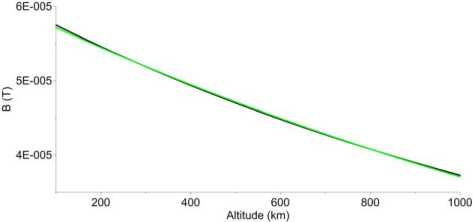
Figure 7 . Height variation (black line) of the geomagnetic field obtained from the IGRF model and its approximation by an exponential function (green line)

the upper limit to consider that t^bHe^–t =0.

The function e^–t in the range of variation of the argument t from [0...10] is approximated by a polynomial, in this implementation we use a polynomial of degree 8:

e ^ at + bt + ct + dt + et + ft + gt + ht + i.

In Figure 8, the approximating polynomial is red. As a result, the problem is divided into three cases: the lower and upper limits are lower than 10; the lower limit is lower than 10 and the upper limit is equal to or greater than 10; both the limits are greater than 10. In the last case, the integral is zero. For the first two variants, the final expressions for the phase are as follows:

Q(r) = aNmF2Hae-br0 x xZ i=0

ai

bH + 1 + i

- ^r 0 h m^F2 ( bH + 1 + i ) - ^r h m F² ( bH + 1 + i )

eHeH если hmF2 < r0 + H ln(10);

Q ( r ) = aN_{n 3}F2 Hae ^{- br} 0 x

x       --- t0 bH +1 + i

10 bH + ^{1 +} i - e

r = h m F2 ( bH + i + i )

,

если h _m F2 >  r ₀ + H ln(10).

Thus, we have derived analytical expressions for the rotation angle of the wave polarization plane, which significantly simplifies the calculations.

In this work, the main focus is on providing stability of the method and its full automation, therefore when calculating the profile of signal fading caused by the Faraday effect we ignored the vertical profile of the temperature ratio and the form of the probe signal. It is not difficult to take them into account in the final version of the algorithm.

DISCUSSION

The method of restoring the N e ( r ) profile from Faraday variations in the signal power profile is used to process regular IISR observations. With IISR in a fully automated mode, we have processed long data series (more than 3700 hours of regular observations) for 2007–2015, which cover all seasons and two solar activity levels — low and moderate. Moreover, in the above range the radar worked in a two-frequency mode, which allowed us to calculate TID characteristics (using data from the Irkutsk ionosonde).

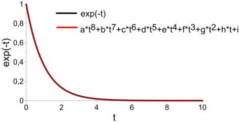
Figure 8 . Behavior of the exponent with a negative argument (red line) and its approximation by a polynomial of degree 8 (black line)

The processing speed is relatively high here: day is processed for less than two hours. Below are the main results obtained with this method.

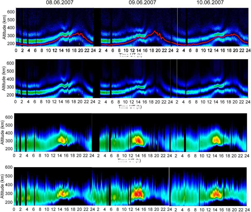
Figure 9 shows the time-altitude experimental scattered signal power profile, recovered profiles of the IS signal power and electron density, as well as the altitude-temporal electron density profile derived from Irkutsk ionosonde data for the June 8–10, 2007 period characterized by low solar activity (the F 10.7 index: 86.8 — June 08, 2007; 81 —June 09, 2007; 78.2 — June 10, 2007). Referring to the Figure, the recovered IS signal power profile repeats with a high accuracy the experimental one, including the observed wave processes. The electron density profile obtained from IISR data has a structure similar to the N e profile recovered from ionosonde data.

An important condition for proper operation of the method is the automatic tracking of the position of the first minimum of Faraday variations in the signal power profile. In the Figure, its position is marked with the red line (data obtained from the algorithm). We can see that the position of the first minimum, found by the automated method, with high accuracy describes that ob- served in the experiment — both in the daytime, with a large number of Faraday variations in the signal power profile, and in the nighttime when there is, in fact, one maximum.

Figure 10 presents the results of comparison between heights of maximum electron density in the F2 layer h m F2 and critical frequency values f o F2, obtained from both IISR and Irkutsk ionosonde data for the same period as in Figure 9. There is good agreement between the behavior of the ionospheric parameters derived from data acquired with both the instruments.

Figure 11 shows the experimental and recovered signal power and electron density profiles for the period of moderate solar activity on October 15–17, 2014 (the F 10.7 index: 125 — October 15, 2014; 138 — October 16, 2014; 144.8 — October 17, 2014). Figure 12 presents results of the comparison between h m F2 and f o F2, obtained with IISR and ionosonde for the same period as in Figure 11.

Time UT h

Time UT h

Time UT h

Time UT(h)

Figure 9 . Altitude-temporal behavior of: experimental scattered signal power (top panel), IS signal powers and electron density recovered from IISR data (second and third top panels), and electron density from Irkutsk ionosonde data on June 08– 10, 2007 (bottom panel)

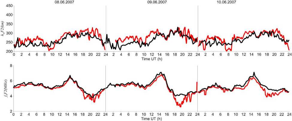
Figure 10 . Time variation of h m F2 (top panel) and f o F2 (bottom panel) for June 08–10, 2007: Irkutsk ionosonde data (black curves); IISR data (red curves)

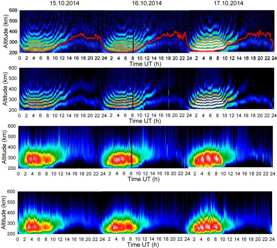
Figure 11 . Altitude-temporal behavior for October 15–17, 2014: of experimental scattered signal power (top panel), IS signal powers and electron density recovered from IISR data (second and third top panels), electron density restored from Irkutsk ionosonde data (bottom panel)

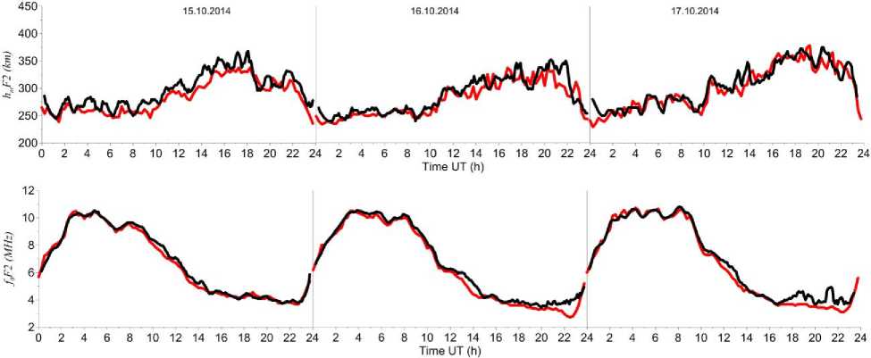
Figure 12 . Time variation of f o F2 (top panel) and h m F2 (bottom panel) on October 15–17, 2014: Irkutsk ionosonde data (black curves); IISR data (red curves)

The comparative analysis also shows good correlation between IISR data for 2014 and ionosonde data. These results show the stability of the method in various heliogeophysical conditions.

Using long data series for 2007–2015, processed with the new method, we carried out a statistical analysis of characteristics of traveling ionospheric disturbances (TIDs) [Medvedev et al., 2013, 2015, 2017] , found climatological features of the mid-latitude ionosphere [Alsatkin et al., 2015] , and calculated the meridional wind velocity with the advanced two-beam technique [Shcherbakov et al., 2015] .

The analysis has shown that most TIDs recorded by the ISTP SB RAS Radiophysical Complex of instruments in a long series of observations of wave-like ionospheric disturbances during solar cycles 23–24 (2007– 2015) are consistent with the concept of propagation of internal gravity waves in the upper atmosphere. Furthermore, the analysis has demonstrated a good correspondence of the electron density obtained in two radar beams and with the DPS-4 ionosonde. This enabled the development of methods for determining the phase difference between TIDs observed with these instruments. In turn, this allowed us to develop a method for determining the full three-dimensional vector and phase velocity of TIDs [Medvedev et al., 2009; Ratovsky et al., 2008] , to obtain representative statistics on TID characteristics, to develop a method for determining the neutral wind velocity, to confirm the filtering of internal gravity waves by the neutral wind [Medvedev et al., 2015, 2017] .

The morphological study of the electron density behavior in the ionosphere, including that above the F2 peak height, carried out over Eastern Siberia for the first time, has revealed a number of regional features; in particular in fall and spring at low solar activity there is a multi-peak structure of the N e diurnal variation.

The application of the new method along with the advanced two-beam technique for determining the meridional wind speed has first allowed us to calculate winds and to carry out the morphological study of the behavior of the neutral meridional wind in 2007–2015 from IISR data. The analysis has shown a good correspondence in the diurnal variation of hmF2 and neutral meridional winds. The comparison between the winds with well-known semi-empirical models has also shown good agreement.

Due to long-term continuous measurements with IISR, we managed to obtain monthly average altitudetemporal electron density variations in the range 180–600 km for four seasons (winter, spring, summer, fall) and two solar activity levels (low and moderate). Considering the data on electron density variations as a quiet ionosphere, we compared them with the simulation results obtained with the Global Self-consistent Model of the Thermosphere, Ionosphere, and Protonosphere (GSMTIP) [Namgaladze et al., 1990; Korenkov et al., 1998; Klimenko, et al., 2006] and with the International Reference Ionosphere (IRI) model [Bilitza, Reinisch, 2008] . We have found that some of the observed features derived from IISR measurements are in better agreement with GSMTIP than with IRI. None of the models reproduces details of the multi-peak behavior of the electron density observed with IISR at 300 km and above for spring (night, morning, afternoon, and evening peaks) and fall (three peaks — day, evening, morning) at low solar activity, but GSMTIP for spring partially reproduces two peaks: morning and day [Zherebtsov et al., 2017] .

Long-term continuous studies carried out with IISR have allowed us to select 337 vertical electron density profiles to compare with the results obtained by the radio occultation measurement method on board the COSMIC satellite, as well as from ionosonde and IRI data [Ra-tovsky et al., 2017]. The comparison was carried out for four seasons and two solar activity levels (low and moderate). There were 10 times more short-term measurements than in previous comparisons between IISR and COSMIC satellite data. As for parameters of the lower ionosphere (maximum electron density and electron content of the lower ionosphere), the differences between COSMIC and ground-based data can be interpreted as errors in COSMIC measurement without significant sys- tematic displacements and with the standard deviation 1.4–1.6 times lower than that of the IRI model. In the case of parameters of the upper ionosphere (electron content of the upper ionosphere and the total electron content of the ionosphere), IRI data on average exceeds COSMIC data by 0.6–0.8 TECU, and COSMIC data is on average higher than IISR data by 1.0–1.1 TECU. The percentage difference between IISR and COSMIC data on electron content of the upper ionosphere may run to 80 %. As for the standard deviation, the COSMIC and IISR data agree better than that from the IRI model.

CONCLUSION

We have developed and successfully tested a new method of restoring electron density profiles from IISR data. Distinctive features of the method are as follows: 1) automatic operation of the algorithm; 2) stability in the range of N m F2 [2·10⁵–2·10⁶ cm^–3]; 3) capability of obtaining results in real time; 4) performance independent of external factors (time of day, season, solar activity level, presence of wave disturbances).

The new method allowed us to process IISR data for 2007–2015. The processed data on altitude-temporal behavior of the electron density enabled: 1) the statistical analysis of TID characteristics; 2) the morphological study of the electron density behavior in the ionosphere over Eastern Siberia; 3) the calculation of winds and the morphological study of the behavior of the neutral meridional wind (using the advanced two-beam technique for determining the meridional wind velocity); 4) the comparison between GSMTIP and IRI data as well as between COSMIC and Irkutsk ionosonde data.

The work was performed with budgetary funding of Basic Research program II.12. The work was performed using the Unique Research Facility Irkutsk Incoherent Scatter Radar [] included in Center for Common Use “Angara” [].