Parallel Algorithms for Freezing Problems during Cryosurgery

Author: Peng Zeng, Zhong-Shan Deng, Jing Liu
Journal: International Journal of Information Engineering and Electronic Business(IJIEEB) @ijieeb
Article in issue: 2 vol.3, 2011.
Free access
Treatment planning based on numerical simula-tion before cryosurgery is an indispensable way to achieve exactly killing of tumors. Furthermore, intraoperative pre-diction based on monitoring results can lead to more accu-rate ablation. However, conventional serial program is diffi-cult to meet the challenge of real-time assistance with com-plex treatment plans. In this study, two parallel numerical algorithms, i.e. parallel explicit scheme and Alternating Direction Implicit (ADI) scheme using the block pipelined method for parallelization, based on an effective heat capac-ity method are established to solve three-dimensional phase change problems in biological tissues subjected to multiple cryoprobes. The validation, speedups as well as efficiencies of parallelized computations of the both schemes were com-pared. It was shown that the parallel algorithms developed here can perform rapid prediction of temperature distribu-tion for cryosurgery, and that parallel computing is hopeful to assist cryosurgeons with prospective parallel treatment planning in the near future.
Bioheat transfer, cryosurgery, phase change, parallel algorithm, explicit scheme, ADI scheme, the block pipelined method
Short address: https://sciup.org/15013075
IDR: 15013075
Text of the scientific article Parallel Algorithms for Freezing Problems during Cryosurgery
Published Online March 2011 in MECS
Cryosurgery is one of the most important therapies for treating tumors. Due to the advantages of hemostasis, painlessness and preventing postoperative infection [1], it has triggered a surge of interest in fields of skin [2], breast [3], prostate [4], liver [5], etc.
Optimal treatment planning strategy is the key factor to cryosurgery. It includes imaging the size, shape, number and location of tumors by three-dimensional image technology, determining the optimal cryoprobe layout (such as insertion paths, depths and the number of cryoprobe), and finally confirming the operative procedure (such as the sequence of insertion and the duration of freezing), all with the help of numerical calculation. Various medical image systems have been used in clinical practice. Nu- merical computing also has facilitated the surgeons’ works. Yet, computing by a conventional serial program consumes a substantial amount of time in prediction, which presents a hurdle for resulting rapid treatment planning, especially involving irregularly shaped tumor tissues and multiple cryoprobes.
Additionally, real-time monitoring during operation, including the size, shape and location of ice ball, for predicting phase change and drawing up further treatment planning is a major goal of cryosurgery but still timeconsuming. It is more sensitive to time.
As above mentioned, the serial program is a hurdle to both the preoperative determination of treatment planning and the intraoperative predication. Instead, parallel computing, which is mature in theory and has been widely applied, is proposed in the current study to enhance computing performance. Explicit scheme is a basic algorithm in parallel computing, since it is easy in comprehension as well as parallelized expediently. However, it is impractical in high-resolution problems owing to severe time step restriction [6]. Alternating Direction Implicit (ADI) scheme is later proposed to overcome this drawback. It is substantially an iterative algorithm, splitting every iteration step into a sequence of one-dimensional, tridiagonal implicit solvers [7], which is relatively easier in parallelization to multi-dimensional implicit scheme. ADI scheme is equivalent to explicit scheme in calculated quantity at certain time step, but it can significantly reduce the overall run time for its avoiding time step restriction by implicitly discretizing partial differential equations.
In this study, two parallel algorithms were developed to accelerate the numerical simulation in threedimensional biological tissues embedded with tumor tissues during cryosurgery. Based on our previous studies [8, 9], we parallelized the serial explicit scheme program on freezing problems associated with phase change and multiple cryoprobes. ADI scheme were introduced thereafter. It is generally acknowledged that ADI can hardly be implemented on distributed-memory parallel computers on account of large amount of data communications. With the purpose to alleviate this difficulty, many methods are proposed, including the transpose strategy [10], fractional steps methods [6], the pre-propagation scheme [11] combined of message vectorization, the block single parallel partition algorithm [12] combined with message vectorization, and the block pipelined method [13, 14, 15]. The block pipelined method can be used to parallelize existing serial programs easily, and coordination between communication and computing can lead to a better speedup [13]. We adopted this method to parallelize ADI scheme and compared its speedup and efficiency with the counterpart of parallelized explicit scheme.
-
II. D ESCRIPTION OF P ROBLEM
-
A. Physical Application
The biological tissue is modeled as a rectangular solid (0.05m x 0.1m x 0.1m), embedded with a cubic tumor tissue (0.018m x 0.018m x 0.018m). The x = 0 surface is skin surface, the x = 0.05 surface body core surface, others are adiabatic surfaces. During cryosurgery, three cryoprobes are inserted into tumor tissues. For the sake of computational simplicity, cylindrical cryoprobes are simplified as cuboids. The boundary conditions at cryoprobe tip and shank are constant temperature and adiabatic boundary condition, respectively. The location of such probes and tumor are listed in Table I .
-
B. Mathematical fomulation and Boundary Condition
Multi-dimensional bioheat transfer by the classic bioheat equation [16] was used in the current work, and the relationship for unfrozen tissues is described as:
C u ^ T u l^ -V' k u V [ Tu ( X , t ) ] - ® b C bTu ( X , t ) + Q m + C b ® b T a (1)
For the absence of blood flow and metabolic activities in the frozen tissues, the energy equation is defined by:
Cf fT^ =V' ^ T f ( X , 1 )] (2)
where Cu , Cf and Cb denote the heat capacities of unfrozen tissue, frozen tissue and blood, respectively; X contains the Cartesian coordinates x , y and z ; t is the time of heat transfer; ku and kf are respectively the thermal conductivity of unfrozen tissues and frozen tissues; ®b is the blood perfusion; Tu , Tf and Ta are the temperatures of unfrozen tissue, frozen tissues and arterial blood, respectively; and Qm is the metabolic heat generation.
TABLE I. L OCATION OF C RYOPROBES AND T UMOR U SED IN
C ALCULATION .
|
Cryoprobes (domain) |
Tumor (domain) |
||
|
Probe tips |
Probe shanks |
||
|
'p |
0.0 ≤ x ≤ 0.016m |
0.016 ≤ x ≤ 0.026m |
|
|
0.047 ≤ y ≤ 0.053m |
0.047 ≤ y ≤ 0.053m |
||
|
0.052 ≤ z ≤ 0.058m |
0.052 ≤ z ≤ 0.058m |
||
|
'p |
0.0 ≤ x ≤ 0.016m |
0.016 ≤ x ≤ 0.026m |
0.012 ≤ x ≤ 0.030m |
|
0.042 ≤ y ≤ 0.048m |
0.042 ≤ y ≤ 0.048m |
0.041 ≤ y ≤ 0.059m |
|
|
0.042 ≤ z ≤ 0.048m |
0.042 ≤ z ≤ 0.048m |
0.041 ≤ z ≤ 0.059m |
|
|
'p |
0.0 ≤ x ≤ 0.016m |
0.016 ≤ x ≤ 0.026m |
|
|
0.052 ≤ y ≤ 0.058m |
0.052 ≤ y ≤ 0.058m |
||
|
0.042 ≤ z ≤ 0.048m |
0.042 ≤ z ≤ 0.048m |
||
According to the principles of phase change [17], temperature continuum and energy equation at the moving interface are given as (hypothesizing that the densities of unfrozen and frozen tissues are same and constant):
T, (X, t) -T, (X, t) - T,(3)
f^ _ «TJX^ = p(4)
fun
-
d n о n
where p is the density of biological tissues, L the latent heat of tissues, vn is the normal velocity of moving inter- face.
Due to highly nonlinear property of the above phase change problem in biological tissue, intricate iteration at the moving boundary is inevitable if directly discretizing the governing equations. In this study, the effective heat capacity method, firstly proposed by Bonacina et al. [18], was applied to avoid this time-consuming work. The advantage of this method is that a fixed grid can be used for the numerical computation, and then the nonlinearity at moving boundary is avoided [1]. The final uniform bioheat transfer equation can be written as:
C5TX ’1) -V-kV [T(X,t)]-abCT(X,t)+Q„ + a%bCT (5) where C% is the effective heat capacity, k% the effective thermal conductivity, Q%m the effective metabolic heat generation, 8%b is the effective blood perfusion. These effective quantities can be defined as follows:
C f , T < T„
T t ) -<
P Qi
C + C
+ f-u , T ml < T < T ,
( T , - T . ,)
I C , , T > T„
" kf . T < Tml k%(T) -J (k, + k, ) /2, Tml < T < Tmu ku ,
" 0,
T > T , T < Tn
Q . ( T ) -^ 0, T„ < T < T ,
mu
I Q m , 0, , « % b ( T ) -b, ® b ,
T > T„
T < Tml
T l < T < T ,u
T > T ,u
where T ml and T mu are the lower and upper phase transition temperatures of tissue, respectively.
Boundary conditions of calculation domain and cryo-
2 t +—A t
3 T i , j , k
^^^^^B
k A t
2 C A y 2
k % A t
2 t +-A t
( T i -1, 3 j , k
^^^^^B
2 t +-A t
2 T i , j , k
2 t +-A t
+ T +1,3 j , k ) =
t + 1 A t
C. Parallel Algorithm
Serial problems can be parallelized by task or instruction. As presented in Fig.1, calculation domain in this study was partitioned into 8 portions ( Block i , i = 1, 8) from middle of every line in accordance by task when there were 8 processors ( P k , k = 1, 8). Each processor owns a portion of calculation domain (a block). Blocks exchange data through inter-block communication by Message Passing Interface (MPI) library.
1) Explicit Scheme
By explicit scheme, (5) expressed in a finite difference form:
2 CAxx1
( T i -1, 3 j , k
t + 1 A t
^^^^^B
3 2 T i , j , k
t + 1 A t
+ T i +1, j , k
) + (1
^^^^^B
8% b C b A t
C %
) T it , j , k
+
k % A t
2 C A x 2
' ( TU, j , k
^^^^^B
2 T t i , j , k
+ T i +1, j , k ) +
( ^Qm + 8% b C b T a )A t
+
k % A t
2 ^C A y1
(T , j -1, k
^^^^^B
2 T t i , j , k
+ T it j +1, k )
+
kAt
( T i , tj , k -1
^^^^^B
2 T it , j , k
+ T i‘,j , k +1 )
t +A t
T i , j , k
k %A t
2 8CAzz
t +A t
'( T - 1, j , k
t +A t
2 T i , j , k
t +A t
+ T i +1, j , k ) =
k ^A t t^ 1 +3 A t 2< C A x 2 ( T i - 1’ j , k
t +1A t
3 2 T i , j , k
t +1A t
+ T + 13 j , k )+(1
a % b C b A t t ^C ~ ) T i ’ j ’ k
vt +z t ,, *b Cb К t 2 kA t 2 k A t 2 k A t^t
T j k = (1 C CAx 2 CAy 2 C A z 2 ) T ’ jk
( Qm + 8ibCbTa ) A t kAt t t
+ C^ + Cw1 Ti - 1, j ’ k + T +1- j ’ k ’
+J%AL (T‘
+ 2 < C A x 2 ( T i - 1,j’k
2 T it , j , k
+ T i + 1, j , k )+
( Q % m + S % b C b T a )A t C %
+ CW ( T*^ -1, k + TJ +1, k ) + ^ ( 4' ’ k -1 + T'
t
, j , k +1
t +2 A t t +2 A t t +2 A t
+ t (Г . 3 , - 2Г. . 3 + Г. . 3
+ 2 C a y 2 ( 1 ’ j - 1, k i ’ j ’ k + 1 ’ j + 1, k )
%
+ 2^ < T itj -1, k - 2 T jk + T itj +1, k )
where Tit , j , k ( i , j , k ) is an approximation of the tempera-
ture at gird point at time t ; A x , A y and Kz are the space
steps in each space dimension; A t and is time step. As above mentioned, it is stable under the restriction:
<% b Cb A t 2 kA t 2 kA t 2 kA t
1 C C A x2 C A y2 C A z2 " 0
It was suggested in (15) that calculation of every interior grid point at certain time step only depends on itself and six neighbour grid points at last time step, which avoids heavy iterative computing. The merit facilitates explicit scheme to be parallelized easily.
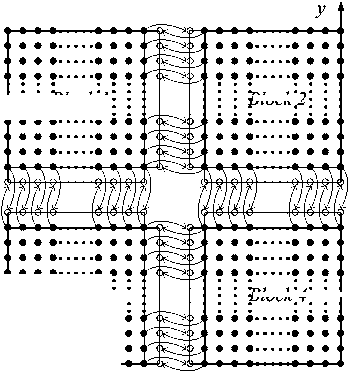
Calculations of interior grid points was distributed by block to corresponding processors, which is independent of grid points of other blocks; border gird points exchanged required data through inter-block communications. Fig. 2 schematically illustrates the message passing process between blocks on a representative cross-section perpendicular to x direction.
2) Alternating Direction Implicit(ADI) Scheme
Peaceman-Rachford (P-R) scheme, Brain scheme and Douglas scheme are the three major ADI schemes for three-dimensional problems, among which P-R scheme is conditional stable but Brain scheme and Douglas scheme are unconditional stable [19]. Douglas scheme was employed in this work, due to its second-order accurate in both time and space [20]. The systems of discretized equations are given as:
t + 1 A t t + 1 A t t + 1 A t t + 1 A t
T 3----- (T .3 , -2T 3 3
T ’ j ’ k %?k\ 2 ( T -1’ j ’ k 2T i ’ j ’ k + T + 1 ' j ’ k )
+ 2 Cz 2 2 ( T ’ j ’ k - 1 - 2 T ’ j ’ k + T '’ j ’ k + 1 )
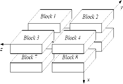
Figure 1. Partition of calculation domain.
k A t
2 CAx 2
( TU j , k
- 2 T tj , k + T M, j , k ) + (1 - ^ b % ) T tj , k
+
k A t
C A y 2
( T it , j -1, k
-
t i, j,k
+ T j +1, k ) +
( Q m + 8% b C b T a )A t C %
z
Block 2
Block 4
Block 3
Figure 2. Message passing for explicit scheme. (a) Solid disks indicate interior grid points inside calculation domain; (b) Hollow circles indicate border grid points for message passing.
Block 1
+
kA t
C A z 2
( T it , j , k -1
-
t i, j,k
+ Ti,j , k +1 )
(17) - (19) can be defined as three systems of tridiagonal equations:
a
variable vector (denote temperature distribution along line); R is the right vector.
In (17), a n =
k % A * r n = " ccat?
k % A t
+ C A y 2 k % A *
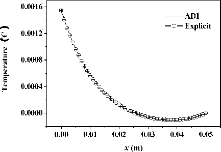
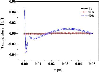
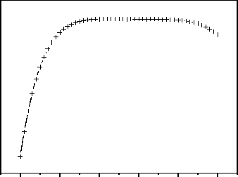
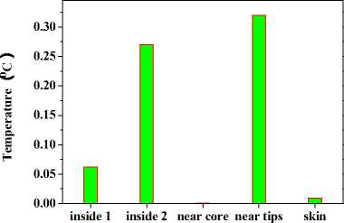
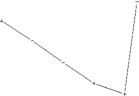
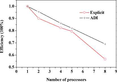
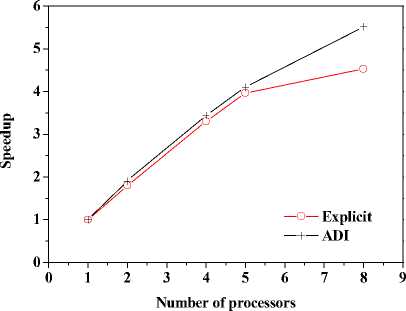
+ - kA * , л kA t 2 CAt2’ bn = 1 +CAt2’ cn •(Tи-1-j-k - 2T*,j k+T*+1-j-k ) + (1- 2 CAt2’ 8 Cb At_t C )Tn.j.k ^^^^B J (T* ТГ- * ^(Qmm + dibCbTa )A* ■(Tn-j ~1-k2Tn-j-k+Tn-j+1-k ) +----------^-------- '(T* ,- ^-1 _2T* : + T T* : b+1 ) (n — 1 ’51). njjs njjs njjs + In (18), an kAt , k%A t ■CCW ’bn =1+C^^y7’ cn ^^^^B J 2 CAy2’ n kAt *+3 A* 2 CAt2 ( и’ n -k ^^^^B t+1a t t+1at 2T n k + T+1-n - k)+a ^^^^B S>b Cb A * * (% ) Ti-n-k r n + 2 CAt2 kAt + 2 CAy2 (T*1-n-k ■ 2T'n-k + T-+1-n-k ) + ■ (T’nB1-k - 2Ti’n-k + T’n+1-k ) (Qm + 8CT )At C + -%AzT(TtnkB1 ■ 2T'n-k + Ttnk+1) (n — 1- 101). In (19), an = kA t , , 2 CAz2’ bn = 1 + ,cn kAt ,/+3A* 2CAt2( ^’j’n ^^^^^B t+-A t t+-A t 2 Tyn + Ti+i,j, n) + (1 ^^^^^в В 2 CAz2’ 8 Cb A t,Tt C) Ti-j-n B kAt t +2CAt2(Ti-j’n j^*- t+j A• 2 (CAy2( i-C1’ n ^^^^^в t +Tt , . (Qm + 8CbTa )At 2Ti- j - n+Ti+1-j - n ) + CC ^^^^^B 22 t+—At t+—At 2T j3 + Ti.j+1, n) + "CCW T■*’n " 2Ti’j-n + T*j+1-n ) +"CCAz?^‘-j-n■* ■ 2T‘j-n + T‘-j-n+1) (n = 1’ 101)' Coefficients for calculation of grid points on boundaries require to be revised in terms of boundary conditions. Thomas algorithm which consists of a forward elimination phase and a backward substitution phase is the classic solution to tridiagonal equations. Two auxiliary vectors ( pi and qi ) for the forward elimination phase are expressed as: ci Pi — T bi i - ai • Pi -1 c1 ri ’ P1= b1 ’ qi = bi ^^^^B B a, • q r —3—, q = 37. (21) ai • Pi-1 b And the backward substitution phase is defined as: Ti—qt - Ti+1 • Pi’Tn—qn. (22) As showed in (21) and (22) the backward substitution phase depends on the results of the forward elimination phase. After block partition processor for calculating second half of the forward elimination have to wait for processors for calculating first half of the forward elimination to finish their computing; reversely the former processors have to wait for the latter ones to finish their backward substitution. Calculation at certain time step did not stop until all grid points are updated by repeatedly implementing this parallelized Thomas Algorithm along each grid line. A whole Thomas process only updated a line of grid point but communicated twice where single communication only send one value; in addition half processors are in idle condition at any time. It is not a good parallel strategy so we introduced the block pipelined method which aggregates a cluster of communications into a single message to reduce unnecessary message passing to obtain better parallel performance. Fig. 3 illustrates the schematic diagram of computing process by means of the block pipelined method in y direction. Calculations in other directions are similar. Communications between blocks are the same as those of explicit scheme. Details of the procedure are listed in Table П. D. Parallel Performance To assess the parallel performance of parallel explicit scheme and ADI scheme for cryosurgery we introduced two basic evaluation criterions in homogeneous computers (The type of CPU size and performance of memory cache and other characteristics are exactly the same): speedup and efficiency [14]. Speedup (Sp ) is defined as: Sp T s . p where Ts denotes computing time that a serial program executed on a parallel computer with the hypotheses that all CPUs are exclusively occupied; Tp indicate the computing time that parallelized program executed by P processors working on P CPUs respectively. Efficiency ( Ep ) is expressed as: Ep — -p-. (24) Figure 3. Schematic diagram of parallel computing process for ADI. (a) Solid cubes indicate interior grid points have been calculated; (b) Hollow cubes indicate border grid points for communication; (c) Solid cylinder indicate interior grid points being calculating; (d) nbx and nbz indicate the size of computing clusters when computation is in y direction. TABLE II. THE CALCULATION OF THE BLOCK PIPELINED METHOD FOR PARALLEL ADI ALGORITHM IN Y DIRECTION. Procedure P4 (Block 4) P2 (Block 2) 1st a) Perform first half of the forward elimination phase in y direction with the size of computing cluster 1 (cube, nbx x nbz). a) Wait. ith a) Send data to P2 for further forward elimination in Block 2 with the size (nbx x nbz) of computing cluster i (cube); b) Perform first half of the forward elimination phase in y direction with the same size of computing cluster (i+1) (cylinder); c) Receive data from P2 for further backward substitution in Block 4 with the size of computing cluster i; d) Finish second half of the backward substitution phase in y direction with the same size of computing i. a) Receive date from P4 for further forward elimination in Block 2 with the same size of computing cluster i; b) Finish second half of the forward elimination phase in y direction; c) Perform first half of the backward substitution phase in y direction; d) Send data to P4 for further backward substitution in Block 4 with the same size of computing cluster i. (n-1)th a) Send data to P2 for further forward elimination in y direction with the same size of computing cluster (n-1); b) Wait. a) Receive date from P4 for further forward elimination in Block 2 with the same size of computing cluster n; b) Finish second half of the forward elimination phase in y direction; c) Perform first half of the backward substitution phase in y direction; d) Send data to P4 for further backward substitution in Block 4 with the same size of computing cluster n. nth a) Receive data from P2 for further backward substitution in Block 4 with the size of computing cluster n; b) Finish second half of the backward substitution phase in y direction with the same size of computing n. a) Wait for calculation in next time step. III. RESULTS AND DISCUSSION In this study, computer codes are parallelized in FORTRAN language linking with MPI parallel library mpich.nt.1.2.5; the operation system is Windows Server 2003; the compiler was using Intel Visual Fortran Compiler 11.1.051; and all the executable programs run on a Symmetry Multiple Processor (SMP) computer, consisting of two quad-core CPUs (Intel Xeon x5365 @3.00Hz) and eight memories (1 GB each). Side lengths of geometrical domain are s0 = 0.5m, s1 =s2 = 0.1m; temperature of tips was first set to Tw = -196 X, and then Tw = 0 X, for comparing the influence of temperature on the calculation accuracy; ambient temperature is Tf = 20 X; convective heat transfer coeffi cient is hf = 10 W / m2 - °C . Other thermophysical properties are listed in Table Ш. TABLE III. THERMOPHYSICAL PROPERTY FOR NORMAL AND TUMOR TISSUES [8, 21]. Thermophysical property Value Unit Heat capacity (frozen) 1.8 MJ/m3 -X Heat capacity (unfrozen) 3.6 MJ/m3 -X Heat capacity (blood) 3.6 MJ/m3 -X Thermal conductivity (frozen) 2 W/m -X Thermal conductivity (unfrozen) 0.5 W/m -X Latent heat 250 MJ/m3 Artery temperature 37 X Body core temperature 37 X Upper phase transition temperature 0 X Lower phase transition temperature -22 X Blood perfusion (normal) 0.0005 ml/s/ml Blood perfusion (tumor) 0.002 ml/s/ml Metabolic rate (normal) 4200 W/m3 Metabolic rate (tumor) 42000 W/m3 Firstly, serial computer programs using explicit scheme and ADI scheme were validated through comparing the results of the one-dimensional analytic solution for a steady bioheat transfer problem of convective boundary at x = 0 and constant temperature boundary at x = 0.5 m (time steps of both schemes were Δt = 0.1s). Fig. 4 and 5 are the comparison outcome. Fig. 4 shows the temperature difference of above numerical solutions and analytic solution, and both schemes have high precision. In addition, the skin boundary is of two-order accuracy in space but core boundary the exact temperature value, thus, values on grid points near core boundary are more accurate. It is indicated in Fig. 5 that there are small numerical differences in results of the two schemes. Numerical results of ADI scheme are more close to those of analytic solution, since Douglas ADI scheme is two-order accuracy in time but explicit scheme is combined with only one-order time discretization. Then, the influence of time step on computing time and accuracy was validated as well. A transient problem on above defined calculation domain was calculated with initial value of 37(the physical time is 1000s). The computing times are given in Table IV; comparisons of accuracy are showed in Fig. 6 and Fig. 7. It is showed in Table IV that computing time is nearly in inverse proportion to time step but in proportion to iteration time. ates once, which is thereby more sensitive to initial stage oscillation. Figure 4. Temperature differences between numerical solution and analytical solution. Figure 6. Comparison of temperature difference respectively by different time steps. 8.00E-011 6.00E-011 4.00E-011 2.00E-011 0.00E+000 i0oaO0=0=™™===0D0[ 0.00 0.01 0.02 0.03 0.04 0.05 u ч^ = 0.4 0.0 -0.4 -0.8 -1.2 -1.6 0.00 0.01 0.02 0.03 0.04 0.05 x (m) Figure 7. Comparison of temperature difference between values by time step being 1000s and 0.1s. x (m) Figure 5. Temperature differences between explicit scheme and ADI scheme. TABLE IV. INFLUENCE ON COMPUTING TIME BY TIME STEP. Different time step Δt (Actual time Tt = 1000 s) 1000 s 100 s 10 s 1 s 0.1 s Computing time (s) 0.28 2.68 26.13 261.14 2536.34 iterations 1 10 100 1000 10000 Fig. 4 has proved the accuracy of one-dimensional numerical results when time step Δt = 0.1s, based on which subsequent tests and verifications of influence of time steps on accuracy are studied. Fig. 6 gives computing results of three time steps (Δt = 1s, 10s and 100s) correspondently subtracting those of time step Δt = 0.1s. The maximal temperature difference are less than 1.0 x 10⁻³oC and 1.0 x 10⁻²oC when time step are 1s and 10s, respectively, which can both be negligible in bioheat transfer. Moreover, the maximum is less than 0.05OC when time step is 100s, which is acceptable. As depicted in Fig. 7, the maximum temperature difference, however, comes up to 1.5OC. In this case, the computing only iter- In this work, we developed a prediction on a threedimensional freezing problem by above mentioned parallel algorithm, and compared their temperature difference of gird points near probes (Table V), normal grid point inside calculation domain (Table ^) and grid points near boundaries (Table TO) when whose freezing temperature is -196 X (liquid nitrogen) or 0 X (saline water). As given in these tables, (29, 50, 55) and (29, 45, 45) are respectively grid points 0.003m front of probe 1 and probe 2; (32, 50, 55) and (32, 45, 45) are grid points 0.006m front of probe 1 and probe 2, respectively; (15, 25, 25) is normal interior grid point near probes, whereas (40, 75, 75) away from probes; (1, 1, 1) and (49, 99, 99) are grid points at skin surface and near core body, respectively. It is given in Table V that temperature difference of such schemes gradually increases and finally levels off, whose time interval from start to stabilization is about 800s. The final stable temperature difference is about 3.2 x 10⁻¹X when the cooling substance inside probes is liquid nitrogen; about 5.4 x 10⁻³X when it is saline water. So computing has a bad but still acceptable outcome in resolution involving relative high temperature (saline water) at tips, which caused by steep temperature gradient between tissues and tips. It can result in high resolution outcome without a great amount of computing when local grid refinement is used around tips [23]. Fig. 6 presents the similar character of normal interior grid points. Nevertheless, the homologous time interval is longer (4000s). (15, 25, 25) and (40, 75, 75) ultimately level off at around 6.2 x 10⁻²oC and 2.7 x 10⁻¹oC, respectively. The similar characters of grid points near domain boundaries are showed in Fig. 7. (1, 1, 1) and (49, 99, 99) are ultimately stabilized at around 6.2 x 10⁻²oC and 2.7 x 10⁻¹oC, respectively. Final aggregated temperature differences of above grid points are given in Fig. 8. Grid points of steep temperature gradient (near tips and inside 2) reveal obvious temperature difference, which results from low mesh density, but is still acceptable; this factor gradually attenuates and its influence diffuses to grid points away from probes (inside 1); temperature difference at skin is primarily affected by discretization of convective boundary condition, whose influence is small on computing; as core body boundary condition is constant temperature condition, there is rarely error of calculation and the difference is only affected by temporal and spatial discretization at its grid point (near core). The size of computing cluster directly impacts the parallel performance of parallel ADI algorithm. A parallel computing was thus developed, with the setting that freezing time is 100s, time step is 0.1s, the number of processors is respectively set to 1, 2, 4, 5 and 8, the relationship of parameters is 2 x nbx = nby = nbz, which indicate the size of cluster. Fig. 9 gives the relationship of computing time and cluster. The overall parallel run time consists of computing time by processors, waiting time and communication between processors. It is shown that the run time firstly decreases with the size of computing cluster. Since computing cluster aggregates a certain number of messages and calculates and calculates by a pipelined way, processors work spontaneously without unnecessary wait and the overall run time is therefore reduced. When nbx drops to 5, the parallel calculation reaches its optimal performance. At this moment, the overall run time is less than the actual physical time, which makes real-time monitoring and prediction possible. When nbx continues to decrease to 3, the overall run time augments markedly. The time cost of inter-block communication becomes the major factor relative to inter-processor waiting cost due to different computing times. TABLE V. TEMPERATURE DIFFERENCES BETWEEN THE TWO Schemes during Cryosurgery (TW = -196X or TW = 0X) at Grid POINTS NEAR PROBE TIPS. Near Temperature Difference x 102 X Probe Tips 20 s 50 s 100 s 200 s 400 s 800 s (29,50,55) 18.60 30.70 36.34 34.02 32.64 31.03 (29,45,45) 17.16 37.42 36.91 33.80 31.49 29.91 (32,50,55) -1.403 12.75 28.07 33.41 34.29 33.20 (32,45,45) -1.542 12.13 28.97 33.95 33.50 32.18 (29,50,55) 1.378 0.893 0.658 0.527 0.473 0.456 (29,45,45) 1.349 0.891 0.657 0.519 0.461 0.440 (32,50,55) 0.344 0.189 0.433 0.471 0.457 0.454 (32,45,45) 0.352 0.174 0.435 0.470 0.452 0.445 TABLE VI. TEMPERATURE DIFFERENCES BETWEEN THE TWO SCHEMES DURING CRYOSURGERY AT NORMAL INTERIOR GRID POINTS. Temperature Difference x 103X , Tw = - ■ 196 X Inside 200 s 500 s 1000 s 2000 s 3000 s 4000 s (15,25,25) 0.795 14.86 36.58 58.07 63.85 62.38 (40,75,75) 0.0565 20.6 112.4 214.2 254.4 268.2 TABLE VII. TEMPERATURE DIFFERENCES OF THE TWO SCHEMES DURING CRYOSURGERY AT GRID POINTS NEAR BOUNDARIES. Near Boundaries Temperature Difference x 104 X, Tw = -196 X 20 s 50 s 100 s 200 s 400 s 800 s ( 1, 1, 1) 63.0 74.2 80.0 84.2 87.2 89.1 (49,99,99) 7.51 7.83 7.91 7.93 7.94 7.96 Figure 8. The final stable temperature differences between the two schemes during cryosurgery (Tw = -196X) at respective grid points. (a) Inside 1: Normal interior grid points (away from cryoprobes); (b) Inside 2: Normal interior grid points (relatively near cryoprobes); (c) Near core: Grid points close to body core; (d) Near tips: Grid points close to cryoprobes; (e) Skin: Grid points on skin. 25 20 15 10 5 0 nbx (nby = nbz = 2 x nbx ) Figure 11. Efficiencies for explicit and ADI schemes with numbers of processors Figure 9. Computing time for ADI with the size of computing cluster. It can be seen from Fig. 10 that speedups of the above two schemes raise with the number of processor. The speedup of parallel explicit scheme is 4.52, as well as 5.52 of parallel ADI scheme, when the processor number is 8. As a result, the performance of parallel ADI scheme is better during this study mentioned three-dimensional freezing problem subjected to multiple cryoprobes. As illustrates in Fig. 11, efficiencies drop with the number of processor. The efficiency of ADI scheme is higher than that of explicit scheme, which is in accord with the results in Fig. 10. The performance of each processor does not enhance with the number of processor due to the restrictions of mounted hardware (CPU), while communication and waiting cost augment with processor. Consequently, the speedups lessen gradually, while the curves of the efficiencies are diametric. Figure 10. Speedup for explicit and ADI schemes with number of processors. IV. CONCLUSIONS In this current work, the explicit scheme and the ADI scheme were parallelized to solve a three-dimensional freezing problem. The results showed that steep temperature gradient, temporal and spatial discretization precision influenced the accuracy of numerical results, where all the temperature results are acceptable. Since explicit scheme is easy for comprehension and parallelization, it was first parallelized to develop a suitable algorithm to accelerate computing. Time step restriction, however, limits its use in high precision computation. Therefore, we then developed a parallel ADI scheme by the block pipelined method. It is showed that whose parallel performance was not only impacted by the partition of calculation domain but also by the size of computing cluster. Results also indicated that its parallel performance was better than that of the parallel explicit scheme. This study introduced parallel computing into cryosurgery, based on which parallel treatment planning is hopeful to assist cryosurgeons to quickly obtain optimal protocols for cryosurgical treatment of complex shaped tumors and to intraoperatively achieve real-time predication. ACKNOWLEDGMENT This work was financially supported by the National High Technology Research and Development Program of China (2009AA02Z414) and the National Natural Science Foundation of China (30770578).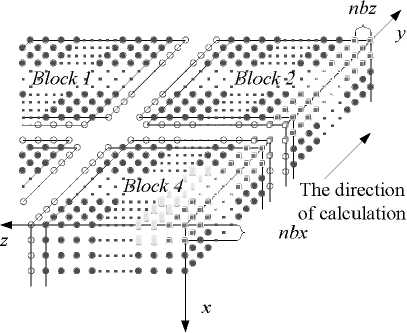

References Parallel Algorithms for Freezing Problems during Cryosurgery
- J. Liu, Principles of cryogenic biomedical engineering, Beijing: Science, 2007. (in Chinese)
- E. G. Kuflik, and A. A. Gage, “The five-year cure rate achieved by cryosurgery for skin cancer,” J. Am. Acad. Dermatol. New York, vol. 24, pp. 1002-1004, 1991.
- E. D. Staren, M. S. Sabel, L. M. Gianakakis, G. A. Wiener, V. M. Hart, M. Gorski, K. Dowlatshahi, B. F. Corning, M. F. Haklin, and G. Koukoulis, “Cryosurgery of breast can-cer”. Arch. Surg. Chicago, vol. 132, pp. 28-33, 1997.
- D. K. Bahn, F. Lee, R. Badalament, A. Kumar, J. Greski, and M. Chernick, “Targeted cryoablation of the prostate: 7- year outcome in the primary treatment of prostate cancer,” Urology. New York, vol. 60, pp. 3-11, 2002.
- R. Adam, E. Akpinar, M. Johann, F. Kunstlinger, P. Magno, H. Bismuth, “Place of cryosurgery in the treatment of malignant liver tumors,” Ann. Surg. Philadelphia, vol. 225, pp. 39-49, 1997.
- M. Krotkiewski, M. Dabrowski, and Y. Y. Podladchikov, “Fractional steps methods for transient problems on com-modity computer architectures,” Phys. Earth Planet. Inter. Amsterdam, vol. 171, pp. 122-136, 2008.
- W. H. Press, S. A. Teukolshy, W. T. Vetterling, and B. P. Flannery, Numerical Recipes: the art of scientific computing, 3rd ed., New York: Cambridge University Press, 2007.
- Z. S. Deng, and J. Liu, “Numerical simulation on 3-D freezing and heating problems for the combined cryosurgery and hyperthermia therapy,” Numer. Heat Tr. A-Appl. Philadelphia, vol.46, pp. 587-611, 2004.
- Z. S. Deng, and J. Liu, “Computerized planning of multiple-probe cryosurgical treatment for tumor with complex geometry,” ASME International Mechanical Engineering Congress and Exposition, 2007.
- T. M. Edison, and G. Erlebacher, “Implementation of a fully-balanced periodic tridiagonal solver on a parallel dis-tributed memory architecture,” Concurrency-pract. Ex. Chichester, vol. 7, pp. 273-302, 1995.
- A. Wakatani, “A parallel and scalable algorithm for ADI method with pre-propagation and message vectorization,” Parallel Comput. Amsterdam, vol.30, pp. 1345-1359, 2004.
- L. Yuan, H. Guo, and Z. H. Yin, “On optimal message vector length for block single parallel partition algorithm in a three-dimensional ADI solver,” Appl. Math. Comput. New York, vol. 215, pp. 2565-2577, 2009.
- L. B. Zhang, “On pipelined computation of a set of recur-rences on distributed memory systems,” J. Numer. Meth. Comput. Appl. Beijing, Iss. 3, pp. 184-191, 1999. (in Chi-nese)
- L. B. Zhang, X. B. Chi, Z. Y. and Mo, R. Li, Introduction to Parallel Computing. Beijing: Tsinghua University, 2006. (in Chinese)
- A. Povitsky, “Parallelization of pipelined algorithm for sets of linear banded systems,” J. Parallel Distrib. Comput. San Diego, vol. 59, pp. 68-97, 2009.
- H. H. Pennes, “Analysis of tissue and arterial blood tem-perature in the resting human forearm,” J. Appl. Physiol. Bethesda, vol. 1, pp. 93-122, 1948.
- M. N. Özisik, Heat Conduction. New York: Wiley, 1980.
- C. Bonacina, G. Comini, A. Fasano, and M. Primicero, “Numercial solution of phase-change problems,” Int. J. of Heat Mass Tran., vol. 16, pp. 1825-1832, 1973.
- W. Q. Tao, Numerical Heat Transfer, 2nd ed., Xi’an: Xi’an Jiaotong University, 2004. (in Chinese)
- J. Douglas, “Alternating direct method for three space variables,” Numer. Math. New York, vol. 4, pp. 41-63, 1962.
- Z. S. Deng, and J. Liu, “Monte Carlo method to solve mul-tidimensional bioheat transfer problem,” Numer. Heat TR. B-Fund. Philadelphia, vol. 28, pp. 97-108, 2002.
- J. Liu, and Z. S. Deng, Physics of Tumor Hyperthermia. Beijing: Science, 2008. (in Chinese)
- M. Rossi, D. Tanaka, K. Shimada, and Y. Rabin, “An effi-cient numerical technique for bioheat simulations and its application to computerized cryosurgery planning,” Comput. Meth. Programs Biomed. Ireland, vol. 85, pp. 41–50, 2007.
