Parameter training in MANET using artificial neural network

Published Online September 2019 in MECS DOI: 10.5815/ijcnis.2019.09.01

Wireless ad hoc networks [1], also known as Mobile Ad hoc Networks (MANET) are self-configuring infrastructure less networks consisting of mobile nodes that can communicate with each other in order to send and receive messages. Nodes in such a network are autonomous [2] and are free to move in any direction and even join or leave the network thus forming highly dynamic topologies.

MANETs differ from traditional wireless networks due to their decentralized system [3]. In a traditional network, nodes send messages to a base station and the base station, in turn, relays these messages to their destination nodes. Thus, these networks are relatively fixed. In MANETs, however, nodes are free to move in any direction and can communicate directly with other nodes by temporarily established links.Fig.1 is an example of centralized wireless network while Fig. 2 shows an ad hoc network [4].

The advent of internet and wireless networks hasmade MANETs a popular area of study. Because of their lack of infrastructure, ad hoc networks have found use ina variety of fields, including environmental monitoring, military communications and disaster relief[5,6]. Due tothe largely dynamic nature of MANETs, efficient routing can be difficult and it has been observed that imposing a hierarchy leads to better scaling [7]. A commonly used routing method is clustering. In our previous paper [8] we have proposed a unique algorithm that chooses efficient cluster heads based on degree of connectivity, battery power and packet drop rate. Our goal in this paper is to extend the previous algorithm by training the parameters used.

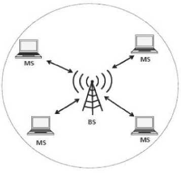
Fig.1. A base station (BS) and its network cell

The proposed model aims to recognize the weights of the factors used in said paper using machine learning, specifically, artificial neural networks (ANN).ANNs are supervised mathematical learning tools inspired by biological neural networks. The network is connected with a vast number of nodes, which are termed as neurons. The connections between the nodes emulate the synaptic connections found in biological entities. In general, ANNs follow the principle of Hebbian Learning [9] which states that the connections between two neurons might be strengthened if the neurons fire simultaneously or, in a more concise way, “cells that fire together, wire together”[10]. Essentially, this means, that neurons which are closely linked with other neurons tend to act on the same input. Since ANNs can be trained to recognize patterns in data, they are incredibly useful for analysis of mapped information. By exploiting this functionality, we aim to create a secure, robust, energy efficient routing algorithm.

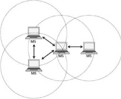
Fig.2. Mobile stations in Ad hoc mode

The rest of this paper is organized as follows: Section II features relevant works. Section III expounds on the principle behind our work. Section IV discusses results obtained and Section V presents our conclusion and discusses future scope of research.

• II.    Related Works

Machine learning has been an integral part of wireless sensor networks since their inception. Machine learning refers to a vast array of methods that help the machine ‘learn’, i.e., progressively improve its performance, to understand and categorize vast amounts of data [11]. The data can either have pre-labeled responses, which is known as supervised learning, or can be unlabeled, called unsupervised learning, where the machine tries to infer meaning from similarities in data points. A number of works have utilized machine learning concepts to develop efficient algorithms for MANETs.

The mobile nature of wireless sensors makes it difficult for researchers to accurately develop schemes for efficient routing, network management, event detection etc. Feng and Chang [12], in their paper, have developed a technique using a hierarchical support vector machine (H-SVM) in order to predict future locations of nodes, as well as, to estimate the amount of noise that will be present in a network so that effective demodulation algorithms can be implemented. The choice of support vector machine was due to it requiring less computation.

A support vector machine can classify n-dimensional data into binary labels by construction of a hyperplane. An H-SVM has multiple levels with a finite number of SVMs [13] on each level that can similarly part the data. Thus, the H-SVM extends the SVM’s ability by being able to classify multi-class data. H-SVM with m levels has 2m-1 SVM classifiers and they are arranged as those 2m-1 branch nodes of a binary tree with height m. According to the authors, H-SVM can classify data in a distributed manner and use simple network information which reduces computational needs. However, the SVM classification error at each stage is assumed to be the same for this work, which will not be the case in real life data. Thus, this model leaves room for error which accumulates at every stage.

Choi and Hossain [14] use a Hidden Markov Model (HMM)[15] to estimate channel parameters in a cognitive radio (CR) system. The goal of the paper is to effectively identify all parameters affecting a channel so that a secondary user (SU) can take advantage of an idle primary user (PU) without hindering any transmission by the PU. Thus, PU traffic pattern, channel gain from PU to SU, and noise density at SU constitute the parameters. Since the PU is modeled as a Markov process, the underlying states representing PU activity is hidden from the SU and the latter can only sense the results. Bayesian learning is utilized to infer these hidden states. Bayesian learning constitutes of deducing the probability distribution of the target variables which are determined using the input sequence. The EM algorithm is used for this task. While this paper identifies a unique approach, it also highlights that the HMM model is not identifiable in some cases due to which the EM algorithm fails. It is also specific only to HMM models and problems must be represented as such for use which makes it non-versatile.

Donohoo et al. [16] have studied a variety of techniques to analyze data from wireless devices in order to predict energy efficient protocols. The list of explored approaches includes linear discriminant analysis [17], linear logistic regression [18], k-nearest neighbor [19], support vector machines [13] and neural networks [20]. Linear discriminate analysis (LDA) used a Bayesian approach. The input data was considered as random variables of a prior distribution. It proved to be a fast and unbiased algorithm, but did not fare well for data with very different underlying covariant matrices. Similar to LDA, linear logistic regression (LLR) is a technique based on Bayes’ theorem which derives a linear model that directly predicts the output variable based on some input variable. However, LLR, unlike LDA, tries to maximize the likelihood of data from a set of classification samples. It is sensitive easy to interpret but possess challenges when the data is complicated.

Support Vector Machine, as we have already discussed, is a powerful scheme which can use multiple attributes to classify data, but is limited to only binary classifications. K-nearest neighbour is a non-parametric unsupervised learning algorithm. It gives fairly accurate results, but is slow and needs all training data at testing phase leading to both time and memory problems. Thus, both these results do not yield much scope for us. Neural Networks on the other hand, showed great promise, getting results with accuracy up to 90%, showing that they perform well where data is imprecise, as is in case of most wireless networks.

Alnwaimi et al. [21] have applied reinforcement learning models to self-configure/optimize femtocells in a distributed heterogeneous network (HN). The HN is represented as a “layer of closed-access LTE femtocells

(FCs) overlaid upon an LTE radio access network”. The FCs, being self-organizing, can sense radio environment and tune their parameters to avoid interference in the network. The model solves resource allocation problems, as well as, interference likelihoods by being able to identify unused slots for spectrum allocation and being able to select sub-channels from the available pool. The authors envisioned that this would lead to better quality of service (QoS).

Gispan et al. [22] uses linear regression to estimate a non-random parameter vector. A distributed network has N sensors which detect some vector v that determines a non-random vector 9. A linear regression model is used for this analysis. For each sensor i, x_; = H 0 + v . The data is compressed before being sent to a fusion center which uses the data to compute the value of 9 . Linear regression is simple, easy to implement, however transferring data to the FC comes at a cost, and while this paper has assumed lossless transmission, that will not always be the case, leading to errors. Moreover, the parameter is computed at one center which makes this algorithm useless for mobile decentralized nodes that are found in MANETs. Such nodes are too dynamic to consider equipping one as a fusion center, not to mention, that back and forth of data transmission would lead to exhausting battery life.

The mobile nature of MANETs make it difficult to obtain efficient routing routes since neighbours continuously keep changing. New nodes are added, old ones removed, or move out of range, and as mobility increases efficiency decreases. To curb this, Cadger et al. [23] devised a novel algorithm that uses machine learning techniques to predict the movement of nodes. The theory was that if the algorithm could predict future locations of mobile nodes, they could plan accordingly and improve overall accuracy. The neural network algorithm was designed and tested using FANN which is an open source C library for creating multilayer perceptron NNs. The authors used 7 input neurons, 15 hidden neurons, 1 hidden layer, and 2 output neurons. Results and data suggest that this algorithm showed considerably positive results and could even be adapted for different parameters. This also suggests that mobility is an important criterion for network topology.

With the recent surge in wireless heterogeneous networks, there has been an increase in utilization of machine learning techniques for finding efficient routes so that nodes can transmit data effectively. Tang et al. [24] have devised a unique approach which deals in controlling traffic in the wireless backbone. Traditional routing protocols do not utilize previously learned data about network congestion to circumvent such problems in the future. Using Convolutional Neural Networks (CNN) the authors aimed to teach the network how to find better routes for their path. The model was evaluated by the authors using extended simulations and was proved to showcase considerably lower delays in delivery time. As previously stated, deep learning mechanism allowed the authors to include varied inputs and allow the model to learn from real world data. This further supports out theory that in a dynamic mobile environment, neural networks are optimum to train data as required.

In our earlier work [8], we have proposed Acceptability Based Routing Protocol (ABRP) which is a secure, hierarchical, energy efficient routing protocol that aims to select cluster heads based on an acceptability score. Acceptability score was calculated as AC = a .D + p .P + / . 5 where, AC is Acceptability Score; α, β, γ are Weight Factors and D, P and S are the number of neighbours, battery power and security factors respectively. While D, P and S differ for each node, the weight factors are selected based on the estimation of their relative importance for the network. This routing protocol works by dividing groups of nodes into clusters and determining a clusterhead to route messages. If the acceptability score of a clusterhead falls below the threshold value defined in the paper, reclustering would be initiated. The drawback of this algorithm was that the values of the parameters, α, β, γ were selected based on their estimated importance. While this algorithm showed good results, we believe it could be further improved by training the parameters using machine learning based on certain input criteria.

• III.    The Proposed Model

In this section we aim to revisit our original algorithm, Acceptability Based Routing Protocol (ABRP) [8] and extend it to be able to determine the best parameters for cluster selection. The goal of this paper is to predict the weight factors for different networks such that the best possible weight factors will be selected. For this, we take characteristics of the netowrk as the input parameters and use artificial neural networks to train the model.

Since ANNs are supervised learning tools, they are incredibly useful in learning patterns with already mapped data. For this project, we have chosen to implement a multilayer perceptron. An MLP is composed of a vast number of connected units arranged in layers. The first layer is always the input layer while the last layer is always the output layer. The inner layers are referred to as the hidden layers and are responsible for the bulk of the processing. MLPs work well when the goal is to map random features to a set output and has good accuracy and speed of learning [25].

In our model, we selected 5 parameters for input, viz, number of nodes, average number of neighbours, mobility, battery power and packet forward rate. A diagrammatic representation of the artificial neural network created as a result is shown in Fig.3. As we have mentioned in [8], battery power and packet forward rate are important parameters for ensuring a low-cost secure routing protocol. Number of neighbours determine the cluster head which is why this parameter has been included. Mobility and number of nodes determine the kind of network we are dealing with [23] and map well to ANNs. The output layer consists of 8 nodes, each having a different α, β, γ combination. Since we know, it is easy to ascertain possible values of α, β, γ using combinatorics. The result was 69 possible cases. These cases included 0

values, a sample of which can be seen in Table 1. Since any one weight factor having 0 relevance would mean that said factor would become irrelevant for our network, we restricted our possible outputs to exclude zero values because all factors are essential. Thus, we re-computed the table eliminating all zero values. This has given us 36 possible factors as seen in Fig.4 that we shall now work with.

a + в + y = 1

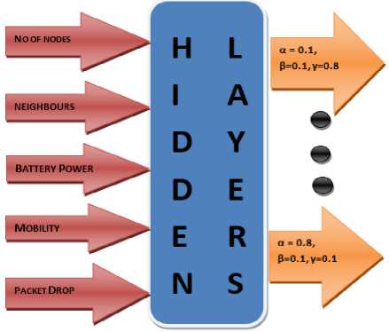
Fig.3. An example of an artificial neural network

Table 1. A sample of possible values of α, β, γ including 0 values.

Serial No	a	p	Y
1	1	0	0
2	0	0	1
3	0.1	0	0.9
4	0.2	0	0.8
5	0.3	0	0.7
6	0.4	0	0.6
7	0.5	0	0.5
8	0.6	0	0.4
9	0.7	0	0.3
10	0.8	0	0.2

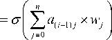
Each node acts as a decentralized processing unit, which, based on its own data activates nodes of the next layer. Traditionally a node is activated by a weighted sum of all its parent nodes. Instead of the binary connections of activation versus no activation we find in biological networks, nodes in an artificial neural network take on probabilistic values. For example, let nodes be denoted by the notation aij where i refers to the layer corresponding to the node while j refers to the node number. Thus, the first node in the input layer will be named a00, while the last node in the same layer will be named a04 for this network. The first node in the next layer will similarly be named a10. The value a10 will be a weighted sum of all the values of its parents, viz, a00, a01, …, a0n where n is the number of nodes in the layer. Since the sum will be greater than one, we use a normalizing function so that the value appears between 0 and 1. In this paper we used ReLU [26] (denoted by a) for this purpose since ReLU has been shown to achieve better result than sigmoid [27]. The weights are the values assigned to the arrows linking each nodes. We use the notation wijk where the arrow connects node j of the layer i to node k of the layer i+1. It is by adjusting these weights, that we determine the strength of the connections and how firing of one neuron will activate the next one. Mathematically, in case of node a10,

I a00- w000 + a01- w010 + a02- w020 | a10 = ^1                                  I         (2)

V ⁺ a 03 ^- w 030 ⁺ a 04 . w 040     )

Where a₁₀ is a node the zeroth node on the first layer and its value is computed by normalizing the sum of all the values in the previous layer multipled with their weights. As we can see, for each node, w_i j _k may just be written as w j . Thus, we can rewrite this equation as

( a 00 - W 0 + a 0! - w 1 + a 02 - w 2 ^a 10 = ^

V + a 03 - ^w 3 + a 04 - ^w 4

In general, aij

Where a_i j is the jth node on ith layer and w j is the weight of the jth node in the i-1 layer. In this manner all the nodes in the ith layer are assigned values. This continues for all successive layers and the neurons keep firing till finally the output layer is activated. Initially, the model starts with generic weights and in each successive case the weights are refined to better suit the predetermined result. A cost function determines how close the result was to the actual value. This process occurs multiple times till the results converge and weights in each layer obtain the best possible value to suit the output. In our case each of the 36 output nodes was assigned a probability value. To train our model, we use a simple mean squared error (MSE) as cost function. MSE is attractive because it is simple to use, parameter free and inexpensive to compute. All lp norms are valid distance metrics in RN, the p = 2 case, in particular, being the ordinary distance metric in N-dimensional Euclidean space [28]. Thus, we compute,

n

MSE = ^ a Lj                (5)

j = 1

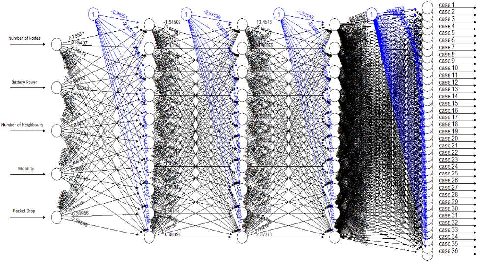
Fig.4. Plot of he neural network formed in R by the algorithm, showing the input parameters, output cases and weights

Where L refers to the last layer, n is number of outputs and â is the expected output value. The sum gives us the total error for the network. For example, if we consider only the first four of the 36 possible cases and assume value 3 is the correct answer, we may get something like Table 2 in the first iteration. The error in this scenario would be the sum of all the squares of differences between observed value and expected value.

Table 2. A simple example for calculating MSE

Serial No.	a	p	Y	Observe d Value	Expecte d Value
1	0.1	0.1	0.8	0.3	0
2	0.1	0.2	0.7	0.2	1
3	0.1	0.3	0.6	0.9	0
4	0.1	0.4	0.5	0.4	0

From this table we can calculate the MSE as,

MSE = ( 0.5 - 0.0 ) 2 + ( 0.2 - 0.0 ) 2 + ( 0.3 - 0.0 ) 2 + ( 0.4 - 0.0 ) 2 = 0.94

Similarly, we calculate MSE for all possible cases and compute the average. With each new dataset, we then try to minimize this cost function using the gradient descent technique [29]. In an n-dimensional space consisting of all the weights and biases, by changing the inputs, we minimize the cost function, and thus, we reduce the error, thereby, allowing the machine to learn. This model consisting of all the parameters is then capable of predicting the best weight factors for our network.

We have used the algorithm from our earlier work to simulate test cases. This has been done using Global Mobile Information System Simulator (GloMoSim) 2.03. In a comparison between GloMoSim, NS2, NS3 and

Omnet++, GloMoSim had the best CPU utilization for large scale networks and was almost comparable to NS3 in terms of memory usage and computational speed. However, NS3 is still considered to be very new and widely lacks credibility. Furthermore, GloMoSim has high scalability and supports much larger networks than NS2 or NS3[30, 31]. The combination of all of these factors led us to choose GloMoSim.

Using this simulator, different scenarios where tested which included different cases of a, P and y. One case was marked as best in each scenario. Metrics like packet drop, number of clusters formed, and residual battery power have aided in this choice. This knowledge was then used to pick five parameters to be used as input, viz., Number of Nodes, Average Number of Neighbours, Average Mobility of Nodes, Battery Power of Network and Packet Drop Rate. The network was implemented using neuralnet package in R, having 5 inputs, 36 outputs and 3 hidden layers with 10 neurons each.

Following this, the results predicted by our algorithm was utilized to simulate networks of different sizes to test our results. Once again, GloMoSim was our simulator of choice. The networks we simulated ranged from 10 nodes to 20. For each case we chose the parameters we had previously selected and the new values. In all cases the training was shown to be effective.

• IV.    Results

The data was divided such that 75% was used for training and 25% for testing. Fig.3 visualizes the neural network used to achieve our results. The input nodes are, as can be seen, are the ones previously mentioned and each of the 36 cases are treated as output. In order to further visualize the data, Fig.5 shows a comparison between real and predicted values that were obtained in the course of our work. The graph thus plotted only shows the cases that were chosen, and not the cases with 0 values in order to keep the plot simple. X-axis

corresponds to the different network configurations test, while Y-axis pertains to the different possible parameter values.

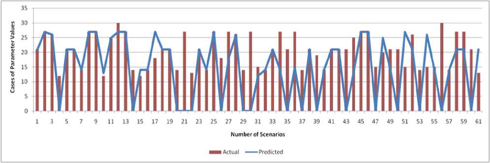
Fig.5. Predicted vs Real Values.

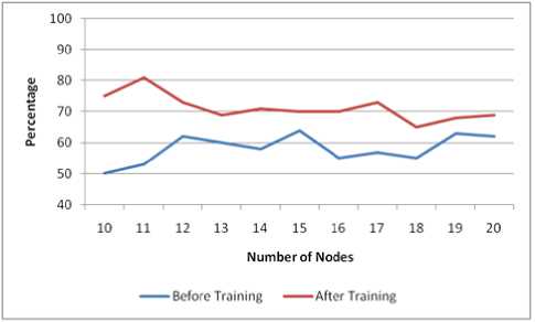
Fig.6. Percentage of battery power in network before data was trained vs. after training

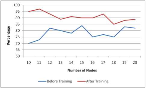
Fig.7. Security factor in network before data was trained vs. after training

A. Accuracy

We denote Accuracy as ACC where

C. Recall

Recall =

ACC =

TP + TN P + N

TP

TP + FN

Where TP= true positive, TN=true negative, P=positiveinstances, N=negative instances. Here, basically the termspositive and negative tells us about the researcher’s predictionor what one can say expectation. True and positive refers tothe fact that whether the prediction is same as that of theobservation.

B. Precision

Precision =

TP

TP + TF

Precision is basically the number of actual positives among those which has been reported as positive.

Recall is the fraction of positives which has been recognized as such.

To determine this, we construct a simple confusion matrix. A confusion matrix is a n x n matrix that is a useful guide to determine the performance of a classifier by tabulating number of predictions inrelation to actual cases. In our case, we will have a 36 x 36 matrix. True

Positive will be all cases where the network predicted 1 and the answer was 1. True Negative will be cases where the network predicted 0 and the actual label was 0. False Positive is when the prediction was 1 but the actual answer was 0 and False negative occurs when actual answer was 0 but the classifier predicted 1.

Using this, we have found that our model displays a 83.3% accuracy. This means that 83.3% of the predicted data was correct. When given information about the

characteristics and topology of the network, our model could accurately predict the best course in most cases. Precision is 75.7% and Recall is 53.2%. Our high precision value shows that the model can correctly recognize a good number of relevant results. Recall results shows that a significant number of data has been correctly identified and that we have been successful in predicting a large number of results. This is good since is shows that our algorithm can be trained to correctly identify the best parameters for our routing protocol

To further verify our results, we have tested our predicted values using GloMoSim. In order to check energy efficiency, we have compared the percentage of remaining battery power in the node for each network with that of the remaining battery power when untrained parameter values were used. This is shown in Fig.5. Security factor was also compared for both cases. Security factor measures the packet drop rate which is used to determine how efficiently packets are transmitted in the network. Fig.6 shows the results. As can be seen in both cases, our current algorithm shows superior results.

• V.    Conclusion

ABRP is a secure, energy-efficient clustering routing protocol which utilizes the infrastructure-less nature of mobile ad hoc networks. The object of this paper was to expand on ABRP and use machine learning techniques, viz., artificial neural networks to train weight parameters -battery power, security factor and degree of neighbours. This algorithm determines the importance of each parameter for a particular type of network in calculating acceptability of a node to become cluster head.

After training, our model was able to analyze input factors like battery power, mobility, packet drop rate, total number of nodes and degree of neighbours in order to correctly predict the best weight parameters for a significant number of cases. The algorithm showed a high rate of success in predicting output values and could accurately identify best weight parameters that would provide the most efficient routing. To determine this, we have further tested the predicted the parameters using GloMoSim. In all cases, training the parameters significantly improved the performance of the algorithm proving the efficacy of our training model. Thus we can conclude that supervised learning techniques, especially artificial neural networks, can be utilized to identify the best routing algorithm for a particular network.

An avenue we haven’t explored is optimizing the number of hidden layers and the neurons present in each layer in order to better predict data. As is obvious, more number of layers increases processing time, which, as the number of data entries increase, could lead to problems. However, too few layers could lead to underfitting. A number of optimization algorithms have also been proposed [32], but wisdom on the subject is varied. Our future work would include determining the best possible architecture of the neural network for greatest efficiency at least cost.