Parameters Nonlinear Estimation of the Propulsion System Performance Seeking Control Using Improved PSO

Published Online December 2010 in MECS

With the improvement of onboard computer performance and the development of control technology, and so on, NASA proposed the conception of propulsion system performance seeking control (PSC) in order to improve the propulsion system performance by exploiting its potential. Some flight tests on F-15 were conducted successfully since 80-90 20th century, and the researches show that PSC can improve fuel efficiency, increase thrust, or prolong engine life, so PSC becomes an important research direction of the aeroengine control fields [1,2].

According to the principle and structure of PSC system, the precise model of onboard engine model is one of the most important parts. PSC consists of estimation, modeling, and optimization, the estimation is the base of PSC. There are some methods to modify the aeroengine model, one direction is to estimate the component deviation parameters (CDP), such as the degraded fan airflow, compress airflow, high-pressure turbine efficiency and low-pressure turbine efficiency, and use the estimated CDP to modify the onboard engine model. This method needs to establish the piecewise linear engine models with the CDP as the additional state variables firstly, which is called state variable model(SVM) conducted from the nonlinear model, then use the Kalman filter and the measurement parameters to estimate the CDP. In all of other estimation process, Kalman algorithm is the key technology of estimation though the estimated parameters are different. Obviously Kalman filter needs linear system model[1-3], but the process of linearizing the nonlinear model will introduce unavoidable errors.

The traditional parameter estimation methods are based on Kalman filter which belongs to linear estimation algorithms and may produce some calculation errors, so the nonlinear algorithm to solve the estimation problem need being researched. According to the model of nonlinear aeroengine with components deviation parameters, the study on utilizing particle swarm optimization (PSO) is carried on, which is a well algorithm for solving the nonlinear equations. The nonlinear estimation of CDP is also based on the measured parameters, but the measurable variables can’t be used directly because of the measurement noises, the testing data preprocessing using Kalman filter is introduced to get the steady measurable parameters. Because of some disadvantages of basic PSO, and the model of the nonlinear estimation is very complex, the estimation results may get into local optimization using basic PSO, an improved PSO is proposed to get more precise results and insure satisfied convergence speed.

• II.    MATHEMATICAL MODEL AND ALGORITHM CHOICE

• A.    The Basic Theory

In terms of researches of NASA PSC, Kalman filter estimation is based on measurement variables and piecewise state variable model, which is conducted from the aeroengine nonlinear model by linearization. But it is not easy to get the full envelope linearized models. Considering that the PSC was designed to operate in steady or quasi-steady-state conditions with fixed throttles[2], the nonlinear estimation method[4] was introduced to estimation the degraded parameters directly based on the nonlinear aeroengine mathematic model including the CDP, which can avoid the linearization error.

As an example, we will establish the nonlinear model of a given engine, which is a low-bypass ratio, twin-spool, afterburning turbofan engine. The estimation of nonlinear parameters is also based on the measured values of measurable parameters. To the degraded aeroengine during operation in steady state, the real measured values and the calculated values of measurable variables should be matched, with which the traditional turbofan engine operation balances compose the fundamental of nonlinear estimation together.

• B.    Nonlinear Estimation Mathematical Model

To the given turbofan engine, the control law is to keep the low-pressure rotator speed constant by adjusting fuel flow. Then the unknown operation variables are:

x e = [ P cL , n H , P cH , ^T 4 , ^dh TH , ^dh TL ]

where P _cL is the fan operation location parameter, n H is high-pressure rotor speed, P _cH is the compressor operation location parameter, T ₄ ^* is the total temperature of combustor, dh_T ^* _H and dh_T ^* _L are the high-pressure and low-pressure turbine enthalpy drop respectively.

The component deviation parameters are:

An = [ A m_f , A m_c , A/ /,, , . , A^ t ]

Where A m^ is the fan air flow deviation value, A m c is compressor air flow degraded value, A ^ HT is high-pressure turbine efficiency deviation value, An HL is low-pressure turbine efficiency deviation value. So the parameters need to be solved are defined as:

x = [ x_e , A 7 ]

As presented above, the engine had to follow the balance principle when the degraded engine operating steadily, the mathematic model of nonlinear estimation is the equations as follows [5].

Continuity equation for air flow at outlet of low-pressure turbine:

err = (M44 - M '4 ) / M44(1)

Continuity equation for air flow at outlet of high-pressure turbine:

err2 = (M40 - M40) / M40

Balance equation for power of low-pressure spool:

err = (NTL — NcL ) / NTL

Balance equation for power of high-pressure spool:

err4 = ( Nth — NcH ) / Nth

Balance equation for static pressure at mixer inlet:

err = (P5 — /^5)/ P(5)

Continuity equation for flow at inlet of nozzle:

err = (P5 — P15)/ P(6)

Where M stands for flow, P stands for static pressure, N stands for power.

Four CDP are chosen, according to the given engine four measurable variables are chosen also: low-pressure spool speed n_L , high-pressure spool speed n_H , high-pressure turbine outlet total temperature Tt ₄₅ , mixer outlet total pressure Pt ₆ . Then four measurable variables matching equations are added to the traditional balance equations:

^err 7 = ( n L , real ^— n L , cal ^{( A} 9 ) ) / n L , real         ⁽⁷⁾

^еГГ 8 = ( n H , real ^— n H , cal ^{( A} 9 ) ) / n H , real       ⁽⁸⁾

e^rr 9 = ( ^Tt 45, real ^{— Tt} 45, cal ^{( A} 9 ) ) / n H , real ^{(9) er}r 10 = ( ^Pt 6, real ^{— Pt} 6, cal ^{( A} 9 ) ) / n H , real ⁽¹⁰⁾

Where the suffix real stands for the true measurement, and the cal stands for the calculation value from the engine model.

Equations (1)-(10) compose the mathematic model of the parameters nonlinear estimation. The CDP estimation was changed to solution of nonlinear equations.

• C.    Estimation Algorithm Choice

Equations (1)-(10) are strongly nonlinear, high dimensional, implicit expressing, sophisticated equations, in terms of the engine operation. The traditional algorithms to solve the system of equations often meet some difficulties, such as needing accurate initial value, the difficulty to get the gradient information, the high probability of getting the local optimization, and so on[6]. The equations set solution can be changed to a single object optimization problem, so the optimization algorithm can be utilized. Genetic algorithm (GA) is a popular evolution optimization method which can solve the difficulties mentioned above. But GA is an optimization algorithm basing searching, the calculation consumption is more than the traditional iteration optimization method, besides the complex operations during the evolution calculation such as crossover, mutation, make the calculation efficiency lower. PSO is developing fast recently, and it can be considered as an optimization algorithm between searching and iteration according to its principle. PSO has some advantages of GA, and is more efficient without complex evolution operations [7], so PSO was employed as the method to solve the nonlinear equations.

• D.    Object Functinon of Optimization

As presented above, in order to use PSO to estimate the CDP, the equations need to be conversed to an object function. The process is given as follows.

Write (1)-(10) as:

err(x) = err(xi,x2,L ,xi0)

= <

' err1( Xi, X 2,L , xn ) err—(Xi,x2,L ,Хю)

M

, e^m (xi, x 2,L , xio)

In terms of the least square principle, (11) are equal to the problem of (12).

min f (x) =—err (x) err (x)

1 10

= “E err2(X1, X 2,L , Xn )

² i = 1

Then the equations set solution is changed to a single object nonlinear optimization problem, which can be solved using the PSO algorithm.

• E.    The Bounds of the Optimization

The basic model of the nonlinear turbofan engine is established based on its component characteristics data, and there are many interpolations during the model calculating. This process can’t extrapolate, because the given characteristics bounds are often the range of engine operating safely. If using extrapolation method, the calculation can give out a result, which only has mathematic meaning, but exceeds the safe operation bounds. So interpolation algorithm is employed, if the interpolation inputs are out of the initial data tables’ bounds, the interpolations can’t continue, and the whole model calculation will break off. If PSO is used to solve the optimization, according to the principle of PSO, when initialize the swarms using random method, unreasonable particles will cause the calculation break off, because the inputs of interpolation out of bounds. So in order to ensure the solution process can be finished without stopping, it is necessary to set the bounds of the variables needing to be solved. According to format of the given component characteristics, the unknown variables are changed to conversion variables. Write unknown variables as [ X1, X2,L , Xi0 ], whose up bounds is Xi ub , and the lower bounds is xi,lb .So the optimization is a constrained problem with bounds:

1 ⁿ

min f (x) =-E err (X1, X 2,L , Xn )

— 7=7                         (13)

s-t- Xi,ub ^ Xi ^ Xiilb , (i = 1,2,L 6)

• III.    M EARSURABLE P ARAMETERS P REPROCESSING U SING K ALMAN F ILTER

In order to get four CDPs, four measurable variables matching equations (7-10) are added to the initial engine traditional balance equations, and there are four measurable parameters in the four equations. If the measurable parameters are steady, they could be used directly. But during the measurement process, the measured values are not steady even if the engine operates steadily, and the measurement noises are included also. So the measured values can’t be used directly, and need to be preprocessed to get the real steady values. We will employ Kalman filter to estimate the steady measured values of the measurements, based on the simple CA (Const Acceleration) model, which is a simplified model.

• A.    The Measurable Parameters Regress on Model of

T mes

Use x to represent the measurable parameters uniformly, and the function x of time t is:

x = x (t)

According to the feature of aeroengine operation procedure, the parameter x can be represented approximately by 2-order Taylor series expansion of t , and the discrete formation is:

_ A t ²

Where A t is the sampling time interval, k stands for the k th sampling time. (15) is the CA regression model of measurable parameters. In fact, many nonlinear problems are approximated by 2-order Taylor series expansions in engineering.

• B.    The Measuralbe Parameters State-Space Equat on and Observat on Eqat on for Est mat on

Kalman filter algorithm is based on linear system statespace model and measurement model. According to the CA model of measurable parameters, the state-space equation is:

x k + i		[ i	A t	A t V /2	[ X k ° l
X k + i	=	0	1	A t	X k	+ w k	(16)
x k 2+i _			0	i	_ Xk\

Where state vector | x k X k x k J stands for X k , X i and &  respectively. X k is the measurement, X k is the time-varying change of rate, and &  is the acceleration.

0       12

w k = I w k    w k   w k I is the system model error.

The observation equation is:

0        12

yk+1 = Hk+1 L xk+1   xk+1   xk+1 J + vk+1

Where v_{k +1} is the measurement error, we will estimate the measurable parameters respectively, so the observation matrix is 1 x 3 dimension:

h. .1 =[10 0

The observation matrix is design in this way is also according to the simplified CA model.

• C.    The Kalman Filter Theory Define a general system as follows:

X k = ф . , k - 1 X k - 1 + W k

Y k = H k X k + e k

Where Xk is state vector, Ф. k-1 is the state transition matrix from k - 1 to k , Wk is the system errors, and ek is the measurement errors. Wk and ek are unrelated discrete white noise, and their covariance matrixes are SWk and Sk . Then the recursion formula of standard Kalman filter is:

Prediction of states： respectively, so the observation matrix is 1x m dimension, and HkSXk HT is 1x1 dimension, which is a const. Then the complex matrix inverse calculation is changed into simple reciprocal calculation, this sequential and separate filter process can improve the filter calculation velocity.

• IV.    I MPROVED P SO A LGORITHM

• A. Basic PSO Algorithm

The basic theory of PSO is that, a swarm consists of m particles which are flying in D -dimension space with some velocities. When searching in flight, every particle updates its position according to its history best position and the global history best position in the defined neighborhood, so the basic expression of PSO is:

V + 1 = ^ V + C 1 R 1 ( P t - X t ) + C 2 R 2 ( P g - X g ) (21)

X t + 1 = X t + V t + 1                     (22)

Where to t is inertia weight, in the basic PSO to t is a constant. C ₁ and C ₂ are positive constants, C ₁ is called individual learning factor, and C ₂ is global learning factor. R ₁ and R ₂ are random value belonging to [ 0,1 ] V_t is the present velocity, X_t stands for the present position, P_t is individual best history position, and P_g is the global history best position in the defined neighborhood [8,9].

^X k = ^Ф . , k - 1 ^X k - 1

^S X_k = ^Ф . , k\ ^S _V k ^Фк,k - 1 ^{+ S} W k

Update observation ：

V k = H k X k - Y k

^S V = ^H-^SH T ^{+ S} k

K k = S . H T ( H.1. H T + S k )^{- 1}     (20)

X k = X k - K k ( H k X k - Yk )

S = S - KH_k S

X _k      X_k      k k X_k

Where K k is the filter gain matrix, S. X is the state prediction covariance matrix [3].

According to the filter recursion formula, if the observation vector are m dimension, a m x m matrix’s inverse, which is ( H _k S X H T + S k ) , needs to be calculated, the calculation consumption is proportion to m ³ . In this paper, we process the measurements

• B.    Design of Time-varying Inertia Weight

Most of the constant in (21) is decided by repeated numerical simulations, of which inertia weight is the most important constant. Inertia weight decides the ratio to inherit the present particle velocity. Usually we need the algorithm to have good exploration capability in the initial phase, and have good exploitation in the latter phase [10,11], that is bigger to in the early phase and the

smaller to in the later phase . So the time-varying inertia weight is designed to satisfy the requirement as equation (23).

to = <

to max

(co max

^{- to} min ) g k

Iter _min

, ^k ^ Iter min

^to min , ^k >  Iter min

Where to and to stands for the maximum and max         min

minimum of inertia weight, k is the present iteration, Iter _min stands for the inertia weight stopping changing.

• C.    Introduce of Constriction Factor

In order to accelerate the PSO convergence, the constriction factor was introduced, and the PSO velocity update formula with constriction factor is:

V.1 = x [®tV + ОД (P - X,)+C2 R2 (Pg - X)]

Where X is constriction factor:

2 k

2 - ф - ф ² - 4 ф

Where ф > 4 , ф = С1 + c2 , К = 1

• V.    S IMULATION A ND R ESULTS A NALYSE

• A.    The Creation of Simulated Measurements.

Firstly, the measurable parameters simulation measurement values should be created as follows:

• •    Four components were set to degrade, the values of CDP were set as:

A m f =1.5%, A m_c =1%, An HT =2%, An LT =1.5%

• •    Substitute them back to the nonlinear aeroengine model to calculate the four measurable variables given above, the calculation values of measurable parameters putting CDP in would be used as the simulated true measurement variables:

n L , real ^, n H , real ^{, Tt} 45, real ^{, Pt} 6, real

• •    Add measurement noise into the measurements according to the measurement sensors.

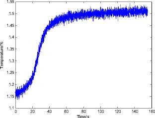
Figure1. Simulation value of measured temperature

According to figure 1, it is obvious that the measurements can’t be used directly, and need to be preprocessed.

• B.    The Example of the Measurable Parameters Preprocess Using Kalman Filter

In order to validate the CA model and Kalman filter for the measurements’ preprocessing, according to the filter algorithm and the measurements’ system model described in section III, the simulated measured parameters are processed. Take Tt _{45, real} as an example also. Set the system errors covariance matrix as 1 x 10 ¹ x I , and the measurement covariance matrix is 3² K ² according to the precision of temperature senor. The initial settings of filter is: the initial values of state variables are set to 0, initial state covariance matrix ^-

Xk is set as 100 x I. (I stands for unit matrix).

The estimation results are given as figure 2 and figure 3. In terms of the results, the estimated values are fit well with the real values, so the estimation results of Kalman filter is satisfied.

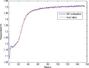
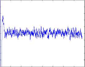
Figure 2. Results of KF estimation

-2

-4

-6

-8

-10

0      20      40      60      80     100     120     140     160

Time/s

Figure 3. Errors of KF estimation

• C.    PSO Algorithm Setting

• •    Learning factors: C 1 = C ₂ = 2.1 ,

• •    Inertia to G [0.4,0.9],

• •    The swarm size is set to a small value: N =25,

V is 10%-20% of X . max                    max

• •    Iteration stopping criteria is set as follows: maximum iterations are set to 800. Epochs before error gradient criterion terminates run are 100. The error tolerance is set to 1e-8.

Simulation of CDP Estimation Using PSO

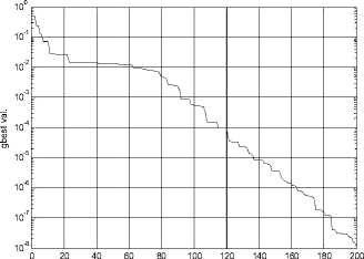
After producing the simulated real measurements, and preprocessing the simulated real measurements, according to the preprocessed steady measurement variables, and the equations set (1)-(10), using the improved PSO algorithm designed in the section IV to estimate the CDP, the iteration process is shown as figure 4-6, and the three figures stand for the iteration process of standard PSO , time-varying PSO and timevarying inertia weight PSO with constriction factor respectively.

According to the converging curves, the result precision of standard PSO is the lowest, which is 10-2 , the precision doesn’t satisfy the convergence requirement, and trap in local minimum. The inertia weight PSO has the satisfied precision of 10-6 , but the converging speed is too slow, the total iterations is up to 700. Only the improve time-varying PSO with constriction factor has both satisfied precision and converging speed, after iterating 160 epoch, the precision arrive at 10-6 .

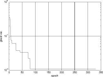
Figure4. The converging curve of standard PSO

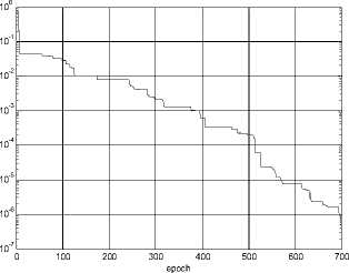
Figure5. The converging curve of time-varying inertia weight PSO

epoch

Figure6. The converging curve of time-varying inertia weight PSO with constriction factor

• VI.    C ONCLUSION AND F UTURE WORK

The estimation of CDP of aeroengine is an important technology of aeronautical propulsion system PSC, the traditional method is to establish the piecewise SVM of the engine in full envelope, and employ linear Kalman filter to get the estimations of CDP. But it is not easy to establish SVM, considering the PSC is designed mainly for the aeroengine in steady or quasi-steady-state operation, so on the base of aeroengine nonlinear steady mathematic model, the CDP were put in, and on the principle of operation balance and measurable parameters matching between the true measurement value and the model calculation value, the nonlinear CDP estimation model was built. The problem was changed to a problem of high-dimension complex nonlinear equations solution, and then was changed to a problem of single objection nonlinear optimization. The Kalman filter is introduced to estimate the measurable parameters, and the precision of estimation is satisfied. The improved PSO is used to solve the problem. The simulation was carried on a given turbofan engine, the calculation results show that PSO can estimate CDP of aeroengine precisely, but the convergence velocity of the PSO designed needs to be improved further. So to improve the PSO algorithm to make the calculation more efficient and to improve the velocity of convergence will be the most important work in the feature.

A CKNOWLEDGMENT

The authors thank Chinese ministerial level fund NO.201089 for its support to our studies.