Partially-Correlated χ2 Targets Detection Analysis of GTM-Adaptive Processor in the Presence of Outliers

Radar has long been used in a variety of military and civilian applications and has become an essential tool of current defensive systems. The chief reason for this belongs to its ability to survey wide areas rapidly during the day or at night and in all weather conditions. Radar systems use modulated waveforms and directive antennas to transmit electromagnetic energy into a specific volume in space to search for targets. Objects within a search volume will reflect portions of this energy (radar returns or echoes) back to the radar. These echoes are then processed by the radar receiver to extract target information such as range, velocity, angular position, and other target identifying characteristics. The primary functions of any radar system are detection, tracking and imaging. The detection process represents the main fundamental concern of the radar because based on it, it will decide to continue or stop any further needed processes.

In attempting to sense the presence of a target through the detection of its returned signal, the radar may have to contend with clutter, jamming, and various interference signals as well as noise. Since both the target signal returns and the radar noise background result from random processes, the detection is a statistical process. This process is accomplished by comparing the received signal amplitude with a threshold level. This threshold is usually set to exclude most noise signals. If the noise power "ψ" is assumed to be constant, then the detection process becomes a simple problem since the detection threshold is held fixed. If the received signal is the larger, a target is declared to be present. Otherwise, it is declared to be absent. In practice, however, the system noise level may change due to changing atmospheric conditions or component temperatures or to a varying noise background from jamming or other interference. In the cases of external clutter and jamming signals, the changes in the noise level and the resulting rate of false alarm may be dramatic. To avoid such situations, many radars employ receiver techniques to compensate for such system noise level changes by continuously updating the detection threshold based on the estimates of the noise variance. The process of continuously changing the threshold value for maintaining a constant rate of false alarm is known as constant false alarm rate (CFAR). Since the CFAR circuits automatically adjust the detection threshold, they have been enthusiastically used in radar systems. As a consequence, much attention has been paid to the task of designing and assessing these adaptive detection techniques since the task of keeping a near-constant probability of false alarm (CFAR) is of primary concern in modern radar systems [1-5].

A target’s radar cross section (RCS), which determines the amount of returned power, varies greatly with the considered aspect angle. Those variations impair significantly the detection and estimation performance of the radar system. Consider a scanning radar system where the antenna's main beam crosses a target. As the beam sweeps past, the radar receives a group of M pulses before the target passes out of the main beam. In some cases cross section is stable enough to produce M constant-amplitude pulses. However, by the time the antenna returns to again search the area containing the target, cross section may have changed. This behavior is characterized by fluctuation from pulse group to pulse group but not within a group. It is sometimes referred to as scan-to-scan fluctuation. Two names, Swerling I (SWI) and Swerling III (SWIII), are usually given to group fluctuations when cross section fluctuates according to the exponential density for case I or the χ2 density for case III. On the other hand, when target cross section fluctuates rapidly enough that each pulse's cross section can be considered independent of the others in a group of M pulses, we say fluctuation is pulse to pulse. Swerling considered this type of fluctuation, which has come to be known as Swerling case II (SWII) for exponential fluctuations of cross section and as Swerling case IV (SWIV) for χ2 fluctuations.

Although Swerling cases bracket the behavior of fluctuating targets of practical interest, recent investigations of target cross section fluctuation statistics indicate that some targets may have probability of detection curves which lie considerably outside the range of cases which are satisfactorily bracketed by those cases. An important class of targets is represented by the so-called moderately fluctuating Rayleigh and χ ² targets, which when illuminated by a coherent pulse train, return a train of correlated pulses with a correlation coefficient in the range 0 <ρ< 1. Partially-correlated χ ² targets have attracted great interest in both theoretical research and practical applications. Therefore, the detection of such type of fluctuating targets is of great importance [6-11].

Target fluctuation lowers the probability of detection,  or equivalently reduces the SNR.

Swerling showed that the statistics associated with SWI  and SWII models apply to targets consisting of many  small   scatterers of comparable RCS values,  whilst the statistics associated with SWIII and SWIV models apply to targets consisting of one large RCS scatterer and many small equal RCS scatterers. Noncoherent integration can be applied to all four Swerling models; however, coherent integration cannot be used when the target fluctuation is either SWII or SWIV because of the de-correlation of the target amplitudes from pulse to pulse  (fast fluctuation), and thus phase coherency cannot be maintained [9].

Since it is of importance for radar processing systems to operate in non-stationary background noise environments with a predetermined constant level of performance, we focus our attention to use the constant false alarm rate (CFAR) algorithm, which sets its threshold adaptively, based on local information of total noise power, to handle this objective of detecting such type of partially-correlated χ2 fluctuating targets. However, potential target information and/or sharp transitions in the clutter power will generally degrade the performance of such detector. To mitigate these effects of outliers, the clutter observations must be censored from large and small deviations. On the other hand, the OS based processors represent the most important category of CFAR detectors due to their immunity to non-homogeneous situations caused by outlying targets and clutter edges [7, 11-14]. These techniques rely on ordering the candidates of a finite-length window devoted to estimate the strength of the background noise and choosing an appropriate reference cell to represent that strength. However, the large processing time taken by it, in scoring the reference samples, limits its practical applications. The modified versions of the OS procedure have been introduced to solve this problem. The GTM algorithm, which is a generalized version of OS technique, has been receiving much attention due to its immunity to outliers as well as its ability to improve the ideal detection performance of the conventional OS scheme [5, 8].

From this brief discussion, it is obvious that there is a need to consider the performance of various CFAR algorithms, which coherently process received signals that are multi-dimensional in nature. In the CFAR context, results of such analysis may be useful in assessing the potential benefits of utilizing the capability of radar systems that can acquire and process multidimensional (or vector) signals. Therefore, our objective in this manuscript is to analyze the performance of the GTM algorithm for partially-correlated χ ² targets with two and four degrees of freedom in the absence as well as in the presence of spurious targets. Section II briefly covers the necessary background information along with problem formulation for the case where the signal fluctuation obeys χ ² statistics with two and four degrees of freedom. The performance of the scheme under consideration is analyzed, in ideal (homogeneous) background environment, and the performance evaluation results are displayed in section III. Section IV is devoted to the performance evaluation along with the numerical results of GTM scheme in multitarget environments. A brief discussion along with our conclusions is outlined in section V.

• II.    S ignal M odel and P roblem D escription

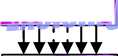
Let us assume that M pulses hit the target which is fluctuating in accordance with χ2 fluctuation model with two and four degrees of freedom. The radar receiver is of superheterodyne type, where the RF stage is a low noise transistor amplifier, in which the mixer and local oscillator convert the RF signal to an intermediate frequency (IF) where it is amplified by the IF amplifier. This IF amplifier is designed as a matched filter; that is, one maximizes the output peak signal-to-mean noise ratio. Thus, the matched filter maximizes the detectability of weak echo signals and attenuates unwanted signals. Almost all radars employ a matched filter or a close approximation. The IF amplifier is followed by a crystal diode, which is traditionally called the demodulator. Its purpose is to assist in extracting the modulating signal from the carrier. The combination of IF amplifier, demodulator, and video amplifier acts as an envelope detector to pass the envelope of the pulse and reject the carrier frequency. This combination is designed to provide sufficient amplification to raise the level of the input signal to a magnitude where it can be the input to a digital computer for further processing. The obtained signal is sampled in range and the sampling rate is chosen in such a way that the successive samples are noncorrelated. The sampled version of the received signal is stored in a shift register of length N+1 resolution cells, where N is an even quantity number. Since the obtained data is collected from M sweeps, the resulting samples can be formulated in a matrix with N+1rows and M columns. Each column of the data matrix consists of the values of the signal obtained for M pulse intervals in one range resolution cell. Let us also assume that the first N/2 and the last N/2 rows of the data matrix are used as a reference window in order to estimate the “noise-plus-interference” level in the test resolution cell of the radar. In this case, the samples of the reference cells result in a matrix X of the size NxM. The test cell or the radar target image includes the elements of the N/2+1 row of the data matrix and it is represented by a vector 0 of length M.

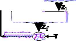
The underlined CFAR detector is shown in Fig.(1). The reference window is applied to a sorting algorithm for the purpose of ordering its elements. The ranked samples go under the processing of excision in order to trim a specified numbers of the lowest and the highest ranked cells before adding the candidates of the reference sub-window to represent an estimation of the unknown noise power level. The estimated noise power levels, from the leading and trailing sub-windows, are then processed under mean-level operation to extract the final noise power level which exactly represents the background noise in the radar receiver. To guarantee a constant rate of false alarm, the average value of the noise power levels must be multiplied by a constant scale value "T" in order to achieve the process of adaptive detection. The result of this multiplication is used as a detection threshold; against which the content of the cell under test is compared in order to declare the presence or the absence of the searching target. Now, let us now go to formulate our problem of detection.

Receiver Noise

Taiiiieinwii™^

1ШШ oring

Vtxcising,

ADDER

ЖШ scoring

Excising

ADDER

Deieciion

Thresholn

Mean-level

M

П

M

II k = 1

1 + ( 1 + ^ S ) Q

П + 1

1 + ^S |n+ 1

2   )

for к = 1

for к = 2

In the above expression, E{.} denotes the expectation operator, S represents the signal-to-noise ratio (SNR), and λ i ’s are the nonnegative eigenvalues of the correlation matrix " Λ" .

In view of Eq.(1), the solution for partially-correlated case requires the computation of the eigenvalues of the correlation matrix Л . It is assumed here that: i) the statistics of the signal are stationary ii) the signal can be represented by a first order Markov process. Under these assumptions, Л becomes a Toeplitz nonnegative definite matrix of a mathematical form given by [8]:

л

■   1	р	2 P         •	M - 2 • P	P M 1
P	1	P^       .    .	_ M - 3 • P	P M - 2
P 2 .	р .	1   .. .    ..	M - 4 • р ..	P M - 3 .
. . P M - 2	. . P M - 3	.    .. .    .. M - 4 ..	.. .. .1	. . P
P M - 1	P M - 2	M - 3 ..	• р	1    _

To simplify the processor performance analysis, Eq.

(1) can be reformatted in a more simpler form as:

Фе<«)

M

п

=1 q + а п в Q + 1

. 1 '    (Q + в )2

with

with

- 1 + Л А

for к =1

в А---¹--- ^к = 1 + Л А /2

for к = 2

It is of importance to note that the eigenvalues for the Swerling III and IV (κ=2) target fluctuation models are the same as that for Swerling I and II cases (κ=1), respectively. Eq.(3) is the backbone of our analysis in the current research. For % ² fluctuation model with four degrees of freedom, the PDF of the output of the i th test tap is given by the Laplace inverse of Eq.(3) after making some minor modifications. If the i th test tap contains noise alone, we let S=0, that is the average noise power at the receiver input is " ^ ". If the ith range cell contains a return from the primary target, it rests as it is without any modifications, where S represents the strength of the target return at the receiver input. On the other hand, if the i th test cell is corrupted by interfering target return, S must be replaced by I, where I denotes the interference-to-noise (INR) at the receiver input.

• III.    S tatistical H omogeneous A nalysis of the GTM P rocessor

In this section, we provide a statistical analysis of the underlined CFAR detector under the condition that the operating environment is free of any outlying targets as well as it represents a homogeneous background. The statistical model with uniform clutter background represents the classical signal situation with stationary noise in the reference window. In this model, two signal cases are of interest: the first case describes one target in the test cell in front of an otherwise uniform background, while the second one deals with uniform noise situation throughout the reference window. In these cases, the background noise has a uniform statistic, i.e., the random variables X1, X2, …...., XN in the reference window are assumed to be statistically independent and identically distributed (IID). In the absence of the target return, the random variable Θ of the cell under test is assumed to be statistically independent of the neighborhood and subject to the same distribution as the random variables Xi’s.

The process of continuously changing the threshold value to maintain a constant probability of false alarm is known as Constant False Alarm Rate (CFAR). This CFAR world of detection assumes that the interference distribution is known and approximates the unknown parameters associated with these distributions. The essence of CFAR is to compare the decision statistic Θ with an adaptive threshold TZ. The threshold coefficient T is a constant scale factor used to satisfy the required false alarm rate for a given window size N when the background noise is homogeneous. The statistic Z is a random variable whose distribution depends upon the particular CFAR scheme and the underlying distribution of each of the reference range cells. Since the unknown noise power level estimate Z is a random variable, the processor performance is determined by calculating the average values of false alarm and detection probabilities. Since the probability of detection is more general than that of false alarm, it is sufficient to compute it in different situations of operating conditions. Actually, the probability of detection tends to the false alarm probability in the absence of the searching target (S=0). Therefore, it is of importance to calculate this interesting characteristic in order to show what its sensing parameters to evaluate them for the processor under consideration. The detailed analysis of this calculation can be found in [6]. Thus, the probability of adaptive detecting a fluctuating target obeying two degrees of freedom % ² model is

P

П^Ф -^{( -} T ^{Q )}, q]

, = 1 Q + a    Q        ^j

i * j

a

a

-

a

Ф - <  T " , )

ij

On the other hand, when the fluctuation of the primary target follows %2- distribution with four degrees of freedom, the probability of detection becomes [11]

P d

M

= E

J = 1

Z

P j

Ф z ( T Pj} + J

"Ф z ( T Pj^

P j

L (Ф z ^{(- T Q)} 1

Where

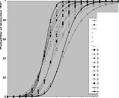
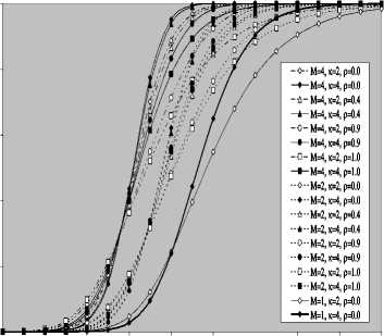
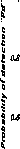
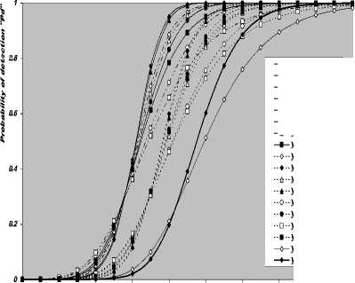
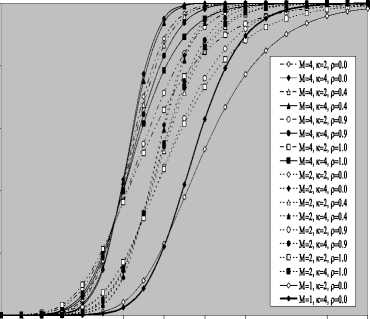
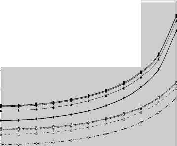
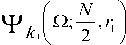
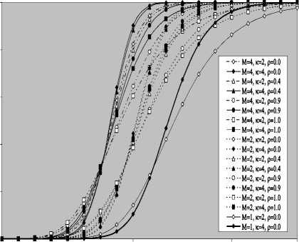
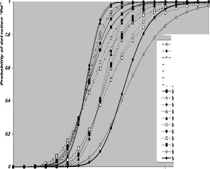
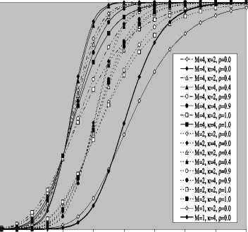
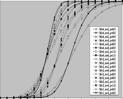
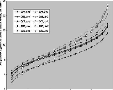
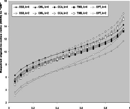
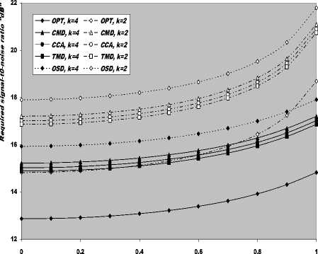
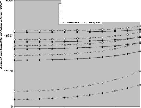
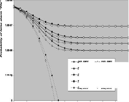
V

Л (1)   Л(2)         Л( к-1)  W( к)  Л( к+1)         Л( n )     ^{v 7}

. M          1 - в

4 А  в,¹ (1 - в,) П вк

i:'      ^{(в - в}

And

А j

M

¹— в,

M

2 E

tjj

The indices in parentheses indicate the rank-order number. X(1) denotes the minimum and X(N) the maximum value. The sequence given in Eq. (10) is called an ordered-statistic. The central idea of the OS- CFAR processor is to select one certain value from the above sequence and to use it as an estimate Z for the average clutter power as observed in the reference window. Thus,

In order to calculate the constant scale factor T for a specified rate of false alarm, it is necessary to obtain the relationship between them. As M-pulse noncoherent integration is used, the required relationship takes a mathematical expression of the form [12]

Pfa

dM-1 [ф(-т Q)'

Q

Q=-1

In this case, Thus,

OZ (Q) has an Mth order pole at Q=-1.

We will denote by OS(K) the OS scheme with parameter K. Practically, the value of K, that maximizes the detection probability of the OS processor in an ideal environment, is generally chosen.

In order to analyze the processor detection performance in uniform clutter background, the statistic of the selected sample must be known. Given that the reference samples are IID, the Kth ordered sample has a PDF of the form [11]:

f (z; N. K) = K f N] [1 - F(z)]N-^K [F,(z)]^K-1f (z) ^{(12) z}OS I к t t t

Pfa

M-1

E j=0

Q=-1

It is of importance to note that the above expression for the rate of false alarm is verified for %² targets either with two degrees or four degrees of freedom. Moreover, the MGF of the noise power level estimate ‘Z’ is the backbone of the processor performance analysis, as shown in Eqs.(4, 5 & 9), either in homogeneous or non-homogeneous background environments. Therefore, our scope in the following subsections is to evaluate this important quantity for the GTM-CFAR detection scheme.

a) Single-Window OS Detector

Since the OS technique represents the fundamental element of the performance analysis of the GTM processor, we will give the basic principles of this procedure that will help us in evaluating the detection probability of the under investigated scheme. To analyze the OS detector, the amplitude values taken from the reference window, of size N, are first rank-ordered according to their increasing magnitudes. The sequence thus achieved has a form

In the above expression, ƒt(.) and Ft(.) represent the PDF and its associated cumulative distribution function (CDF) of the sample that contains thermal noise return, which is uniform and of background clutter power ψ. This PDF has a MGF given by Eq.(1) after setting S equals zero. The Laplace inverse of the resulting formula yields

U(z), in the above expression, denotes the unit-step function. The integration of the above equation gives its associated CDF which becomes

M-1

F, (²) =¹- E

=0

exp(- z)U (z)       (1

(L ⁺ 1)

ф₇(Q;N,K) ZOS

K

Г(М)

Г N 1

VK '

у Kc - Pi

E I • I (-1) K^-i^-1Ф t(Q, i) i=0 V i )

MM

Y A M + _E(i-1) 9   & _E9 = N - i - 1

i=2                               j=1

where

N - i-1 N - i-1

Ф,(Q, i) A E E

91=0 92=0

N - i-1 . E 9m=⁰

П ------------5" ^r(N - i)

,' (f(9, +1) [Г(q)]⁹)

Г(в) (Q+N - i)^r

With

Once the MGF of the noise power level estimate (ZOS) is obtained, the processor detection performance becomes an easy task as we have previously demonstrated. Finally, the ℓth derivative of this MGF is given by

d— {ф  (Q; N, K)} = -K- d Q    Z OS        )    Г( M )

K-1

E i=0

(-1)^K-■^-1

N - i-1 N - i-1

EE

91=o 92=0

N - i-1

E

9m=0

M

Ш

r(9q +1) [Г( q) ]⁹q

^Г(^N -i )^

(-1/ (y),r(Y) (Q + N - i) ^YY+

The notation (γ)ℓ represents the Pochhammer symbol which is defined as [13]

( Y)    A ^{1 (Y +}) = j

VP  = Г( Y)     [y (Y+0(y+2).

for ^ = 0

.( y+^-1)     for ^>0

A desirable CFAR scheme would of course be one that is insensitive to the changes in the total noise power level within the cells of the reference window so that a constant rate of false alarm can be achieved. This is actually the case of all the architectures considered in this manuscript.

• b)    Single-window GTM Detector

A more generalized OS-CFAR detector, which combines ordering with arithmetic averaging, is discussed in this subsection. Such a scheme is known as trimmedmean (TM) filtering in signal processing literature. This processor has a performance which is the best compromise between homogeneous and non-homogeneous operating environments. In this processor, the ordered range cells of a particular reference window are trimmed from both the upper and lower ends. The threshold is estimated by forming the sum of the remaining range cells. The linear combination may be anticipated to give better results because averaging estimates the noise power level more efficiently as in the case of cell-averaging procedure.

The TM scheme first orders the candidates of the reference window in an increasing magnitude and then trims N1 cells from the lower end and N2 ones from the upper end before summing the rest to estimate the unknown noise power level. In other words, the construction of ZTM takes the form [3]

ZTM

A

N^-N 2

E

£=N₁+1

X(<)

The CA and OS(K) schemes can be treated as special cases of this processor with (N1, N2) = (0, 0) and (K-1, N-

K), respectively. In order to include the other familiar CFAR schemes, as special cases, the generalized trimmed-mean (GTM) algorithm has been introduced [5]. The statistic of this new version has a form given by

N-N₂

Zgtm a Ex,,, + nx(N-N2)  <21> j=N1 +1

η, in the previous formula, denotes to weighting factor. This factor is chosen in such a way that the processor mechanism will lead to unbiased estimate of the unknown noise power level [2]. We will denote the GTM-CFAR processor, with N1 trimmed samples from the lower end, N2 censored cells from the upper end and a weighted parameter η, by GTM(N1, N2, η). Based on this definition, the well-known CFAR schemes can be considered as special cases of this new version of GTM processor. They can be defined by assuming specific values for its parameters according to Table (I).

Table 1. Trimming Parameter Values For The Well-Known CFAR Processors

Parameter Algorithm	N1	N2	η
CA	0	0	0
OS(K)	K -  1	N - K	0
CCA(K)	0	N - K	0
CML(K)	0	N - K	N - K
TM(T1, T2)	T1	T2	0

To start the analysis of this more generalized version of the TM detector, it is of importance to note that the ordered statistics X(1), X(2), …….., X(N), are neither independent nor identically distributed even when the original samples X1, X2, ……., XN, are IID random variables. However, when the observations are exponentially distributed, the clutter variates Xi’s can be transformed into another independent random variables Yℓ’s, ℓ=1, 2, ……., N-N1-N2 according to the following relation:

_д     |Х( .1 +1)                   for      ^ =1

^{Y   =}   |X₍.1+0- Х( .1 +м)   for    ²«< . - .1 - .2

In terms of MGF’s of the ordered-statistics X(i)’s, we can compute the Laplace transformation of the previous expression to obtain the MGF of the random variable Yi which becomes [3]:

	[Фх  (®) x( .1+1)	for	£ = 1
Ф Y (®)  = ‘	фу  (®) x( .1+/) фу   (®) [ ^X,.1+2-1)	for	2 <£<.-. - .2

Since the MGF of the ℓth ordered statistic X(ℓ) represents the backbone of the calculation of the corresponding MGF of Yℓ, we are going to evaluate it. This MGF is given by Eq.(15) after replacing K by ℓ. Thus, ф (Q;. ,^ = X и

(.)

Г( M )UJ

4-1 (е-1)

^SI i j

НГ

. - i-1 . - i-1

S S j0 =0 j =0

.^^{1 B(}.  i  1;^j₀,^j1,,'m-1)

S      m -j

-"-'=•        П[Г( p + l)]'p p=0

/ M-1

^Г| S mjm^{+ M}

V m=0

( m-1         )

(^ Q + . - i )Г1 mS0 mjm + M j with

	' r(L +1) M	if	M L=S^
B( L ;^Л,M)   A   «	Пг(м 0 i=1 I0	if	i=1 M L *S- (25)
In terms of Yi’s, the	noise power	level	estimation

ZGTM, given by Eq.(21), can be written as

NT

Zgtm = S(^NT +n-^+1) Y , .TA .-.2-.1   ⁽²⁶⁾

£=1

Since Y_i’s are statistically independent, the MGF of ZGTM can be easily obtained by multiplying the individual MGF’s of its associated random variables. Therefore, we have

N_T

Ф₇(п) = П Ф (^Q)

Z GTM                Y п=( NT + n-^ + 1)п

Once the MGF of the noise power level is calculated, the detection performance of the CFAR processor under consideration is completely determined.

• c)    Double-window GTM Detector

Although the ordered-statistics based detector has some advantages over the conventional cell-averaging scheme, the large processing time taken by it in sorting the candidates of the reference window limits its practical applications. The double-window detector has been introduced as a solution to this problem [5]. Employing two simultaneously specialized processors, one for each set of neighboring cells, it is possible to reduce by half the single-window processing time without altering the estimation of the clutter statistics. On the other hand, if the leading and trailing sets of cells are independently ordered and subsequently compared under the mean, the maximum, or the minimum criterion, we will obtain a new random variable with differing statistics from the representative cell of the OS-CFAR algorithm. Each one of these modified versions can reduce the single-window processing time in half and has the same advantages as the OS detector with only a negligible increment of the CFAR loss. Since the mean-level (ML) has the best compromise performance when the operating environment is either free of or contaminated with spurious target returns, it is of importance to be interested in evaluating the performance of the ML-GTM algorithm.

Referring to Fig.(1), the elements of the reference window are equally partitioned into leading and trailing sub-windows. The generic operation of the two-window family of CFAR schemes is to process the cells of each local sub-window separately, and then combining the resulting estimates through the ML operation to obtain the final estimate of the unknown noise power level. The samples of the leading sub-window (of size Nh=N/2) are firstly ordered from smallest to largest and then the L1 cells are discarded from the lower end and the L2 ordered samples are trimmed from its upper end before adding the rest ordered cells to estimate the unknown noise power level of this sub-window Z₁. Therefore, the estimation of leading subset noise power level is given by

.h - L2

Z1 ^A^^{S X}(₀^{+ П1 X}(.h -L2)  ⁽²⁸⁾

Similarly, the estimation of the noise power level of the trailing reference sub-window Z2 is

Nh - T2

Z 2 A X ^X(j⁺П2 j=T1 +1           '

- T2 )

Here, the smallest T1 ordered samples and the largest T2 ordered ones are excised from the candidates of the trailing subset while the rest cells are added to formulate the noise power level estimate of the sub-window under consideration.

In the ML-GTM processor, the total noise power is estimated by combining the local noise level estimates through the mean operation. The combiner puts out the noise level estimate Zf as

Zf a 1 X Z ²    1=1

The rationale for the mean family of CFAR schemes is that by choosing the mean, the optimum CFAR detector in a homogeneous background when the reference cells contain IID observations can be achieved. In addition, as the size of the reference window increases, the detection probability approaches that of the optimum detector, which is the object that each processor tried to attain its behavior.

Since the total noise power level estimate is obtained by averaging the local estimates of the noise power estimates, the MGF of Zf is simply given by the product of the MGF’s of Z₁ and Z₂. Therefore,

Ф^ (Q)

Zf

П Ф  (Q) (31)

£ =1       Ze

By following the same steps as in the case of singlewindow detector, we can derive the MGF of the leading subset noise power level estimate Z1, where the ℓth ordered cell has a MGF given by

Ф (Q; Nh, £) =

^X<-)

f Nh к p^-1 r(M) U J ^XV i ,

Nh - i-1 Nh - i-1

X X j0 =0  j =0

Nh — i—1 . X ^jM -1 =0

^{B (}Nh^-i^{-1; j}0, Ji,......, ^jM-1)

M-1                .

n=0

Г X mj. + M

V m=0

(^ q+N - i )^гl mj

And

Lt

Z1  = X (Lt +П1 -k +1) Yk ,  Lt A Nh -L2 - L1

k=1

Where

Yk  A

'X(L,)                    for^k = 1      (34)

^X(L+ k-1) -  X(L+ k-2)   for²^^k^^Lt

Similarly, the trailing noise power level estimate Z₂ has an expression of the same form as that given by Eq. (33) after replacing L , L2, η1, and Lt by T , T2, η2, and Tt, respectively. Thus,

Tt

Z2 = X (T. +П2 -k +1) Yk , T_t A Nh -T2 - T1

k=1

Again, we demonstrate that once the MGF of the noise power level estimate is obtained, the processor false alarm and detection performances are fully determined. Finally, a desirable CFAR scheme would of course be one that is insensitive to changes in the total noise power within the candidates of the reference window so that a constant false alarm rate is maintained. This is actually the case of our selected algorithm.

• d)    Processor Performance Assessment

In this subsection, some numerical results are presented to verify the above analysis and compare the performance of the GTM family under ideal operating environments. In other words, the numerical evaluation of the above derived formulas is carried out to obtain an idea about the behavior of different detection algorithms against the strength of correlation between the target returns. The displayed results are the outcomes of a computer program the input data of which are: the size of the reference window (N) is taken as 24, the design false alarm rate (Pfa) is chosen to be 10-6, the number of sweeps (M) varies from 1 to 4, and the correlation coefficient of the primary target's returns (ρs) is allowed to vary from 0 to 1; with special focusing on its initial and final boundaries. Figs. (2-6) depict the detection performance of the family of GTM-CFAR scheme for partially-correlated χ2 fluctuating targets with two and for degrees of freedom when the radar receiver integrates two and four consecutive sweeps and operates in an environment which is free of any outliers. This family incorporates the well-known processors: CA, CML, CCA, TM, and OS, respectively. Similar parameter values, for the leading and trailing sub-windows, are assigned in running our computer programs. For the comparison to be clear, we choose the optimum value for the ranking parameter K which is 10 for Nh=N/2=12. Since the two noise level estimates are combined through the mean-level operation and this is common for all the candidates of GTM-CFAR scheme, it is sufficient to call each detector with that rule based on which the noise level is estimated. Fig. (2) displays the detection performance of GTM(0,0,0) processor. In this case, the local noise level is constructed based on the CA formula: N1=0, N2=0, and η=0; as Table (I) demonstrates. To see to what extent the M-sweeps can improve the detector performance, the single sweep (M=1) results are also included in all the family of curves. It is of importance to note that the candidates of this scene are labeled in the number of sweeps (M), the degrees of freedom (k=2k), as well as the strength of correlation between the target's returns. The behavior of the curves of the underlined figure illustrates that for weak signal return; the more correlated samples give higher performance than those of weak correlation. As the signal strength becomes highly, the two behavior cases approach each other till the point at which the two performances coincide. The continuity of the signal strength makes the reverse of the above behavior to be satisfied, where the weakest target's returns presents higher detection performance than those of strong correlation among them. In other words, there is a critical value of SNR; before which the processor's performance improves as the correlation of the samples increases, whilst the detector's behavior deteriorates, behind that value, as the correlation of the reference samples augments. Additionally, all the partially-correlated curves are always embraced by the Swerling's models which represent the initial (ρs=0) and the final (ρs=1) values of the correlation coefficient between the returned samples of the primary target. This behavior is common either in the case of target fluctuations obeying χ2 with two degrees of freedom or in the situation where the target fluctuates following χ2 statistics with four degrees of freedom. However, the performance corresponding to χ2 statistics with four degrees of freedom is always higher than that obtained for χ2 distribution with two degrees of freedom; given that all the parameter values are held unchanged in the two situations. Additionally, the critical point is the same for the two situations of target fluctuations. Moreover, as M increases, better performance, and consequently lower CFAR loss [7], is obtained for the two cases of target fluctuations, given that the parameter values rest unchanged.

-5        -1        3        7        11        15       19       23       27       31

Primary targetsignal-to-noise ratio (SNR) in "dB"

• ■ M=4, k=2, p=0.0

• - M=4, k=4, p=0.0

• - 4-M=4, k=2, p=0.4

• - 4- M=4, k=4, p=0.4

• - «-M=4, k=2, p=0.9

• - •- M=4, k=4, p=M

• - o-M=4, k=2, p=1.0

M=4, k=4, p=1.0

M=2, k=2, p=0.0

M=2, k=4, p=0.0

M=2, k=2, p=0.4

M=2, k=4, p=0.4

M=2, k=2, p=0.9

M=2, k=4, p=0.9

M=2, k=2, p=1.0

M=2, k=4, p=1.0

M=1, k=2, p=0.0

M=1, k=4, p=0.0

-5         -1         3         7

11       15       19       23       27       31

Primary target signal-to-noise ratio (SNR) in "dB"

Fig.(3) shows the variation of the detection probability of GTM(0,2,2) scheme as a function of the primary target signal strength for several values of M when the target returns have a correlation of 0, 40%, 90%, and 100%. This processor is known in the literature as CML scheme. The local noise level of CML is achieved by adding up the cells of the reference window after ordering them and rejecting the two largest ones and adjusting the weight of its top ranked sample according to the rules of Table (I). The carefully inspect of the curves of this figure demonstrates that they vary in the same manner as those of Fig.(2) with minor degradation and their behavior is identical to the previous detector. This procedure of detection gives the best homogeneous performance after the conventional CA processor. Fig.(4) displays the same thing for GTM(0,2,0) scheme in which the local noise level is extracted by adding up the lowest ordered N/2-2 samples and this is equivalent to the CCA processor. Fig. (5) illustrates the variation of the detection probability with the strength of the primary target's signal for GTM(4,4,0) procedure in which the estimation of the local noise level is carried out by summing the middle four ordered samples after excising the four lowest ordered cells and the four highest ordered ones and this is equivalent to the conventional TM detector. Fig.(6) depicts the same thing for GTM(9,2,0) detector in which the local noise level is estimated by selecting the tenth ordered cell and this is equivalent to the conventional OS detector. The results of these figures show that the detection performances of all the processors under investigation behave the same behavior with minor distinction from one detector to another. In each figure of this family, there are two families of curves: the first one represents the detection performance of the processor under investigation for partially-correlated χ2 targets with two and four degrees of freedom when the correlation strength of the target's returns takes the values ρs=0, 0.4, 0.9, and 1.0 for the case where the number of integrated pulses is 2, and the second family indicates the same performance when the processing data are the results of 4 integrated pulses. At low values of SNR, the detection performance improves as ρs increases and the SWI model gives higher performance than SWII case when the fluctuations of the target obey χ2 distribution with two degrees of freedom, whilst SWIII case has the top detection performance than the SWIV model in the case of target fluctuations with four degrees of freedom for the χ2 statistics. This behavior is rapidly changed as the signal of the primary target becomes stronger where the processor performance attains its highest value for ρs=0 (SWII model for κ=2 or SWIV model for κ=4) while its lowest value is achieved for ρs=1 (SWI model for κ=2 or SWIII model for κ=4). In other words, the Swerling models embrace the correlated curves either the primary target's signal is weak or strong. For comparison, the single sweep detection performance is incorporated in these figures to show to what extent the processor performance improves as the number of integrated pulses augmented. Examining the curves of this group of figures demonstrates that as ρs increases from zero to unity, more per pulse average SNR is required to achieve the same value for the probability of detection. Additionally, for fixed SNR, there is an improvement in detection performance as the number of integrated pulses increases and this is common for all the processors considered here.

0.4

0.2

-5        -1         3         7        11        15        19        23        27        31

Primary targetsignal-to-noise ratio (SNR) in "dB"

0.8

-5        -1        3        7        11        15        19       23       27       31

Primary target signal-to-noise ratio (SNR) in "dB"

-•о- М=4, к=2, р=0.0 -♦— М=4, к=4, р=0.0 -Ь- М=4, к=2, р0.4 -*- М=4, к=4, р=0.4 -О- м=4, к=2, р=0.9 -е- М=4, к=4, р=0.9 -а- М=4, к=2, р=1.0

М=4, к=4, р=1.0 М=2, к=2, р=0.0 М=2, к=4, р=0.0 М=2, к=2, р=0.4 М=2, к=4, р=0.4 М=2, к=2, р=0.9 М=2, к=4, р=0.9 М=2, к=2, р=1.0 М=2, к=4, р=1.0 М=1, к=2, р=0.0 М=1, к=4, р=0.0

0.4

-5        -1        3        7        11        15       19       23       27       31

Primary target signal-to-noise ratio (SNR) in "dB"

19 h

ё

OPT, K=2

GTM(0,0,0), K=2

GTM(0,2,2), K=2

GTM(0,2,0), K=2

GTM(4,4,0), K=2

GTM(9,2,0), K=2

OPT, K=4

GTM(0,0,0), K=4

GTM(0,2,2), K=4

GTM(0,2,0), K=4

GTM(4,4,0), K=4

GTM(9,2,0), K=4

0.6                    0.8                     1

Corelation coefficient "р"

Fig. 7 M-sweeps required SNR, of GTM family of CFAR schemes, to achieve an operating point of (1.0-E6, 0.9) for N=24 and M=3 when it operatesin an ideal environment

To gauge the performance of GTM-CFAR algorithms for finite observations and to compare their behavior against the uniform distribution of clutter throughout the elements of the reference window, the required SNR, to achieve an operating point of specified values for the detection and false alarm probabilities, is taken as a figure of merit. This important parameter is chosen to examine which processor has the top performance and which one gives the worst behavior against the detection of fluctuating targets obeying in their fluctuation to χ² distribution with two and four degrees of freedom. Fig.(7) depicts the variation of the required level of signal strength as a function of the correlation coefficient between the primary target returns for a constant level of detection of 90% as well as a fixed rate of false alarm of 10^-6 if three consecutive sweeps are noncoherently integrated (M=3). Both types of target fluctuations (к=2 & 4) are taken into account in plotting the curves of this figure. As a reference, against which any processor performance is compared, the results of the fixed-threshold detector under the same operating conditions are included among the curves of this figure.

The displayed results show that the required SNR remains approximately constant till the correlation coefficient reaches 60%. After that specified value, there is a noticeable increase in the signal strength as the correlation of the target returns increases. On the other hand, the demand signal level, to satisfy the pre-assigned values of the detection and false alarm probabilities, attains its highest value when the target returns become fully correlated. This behavior is common for all the considered algorithms including the optimum processor. In addition, the correlated returns from target fluctuating according to χ²-distribution with 4 degrees of freedom requires less signal strength than those coming from fluctuating target obeys χ²-statistics with 2 degrees of freedom. The curves of this figure illustrate that the GTM(0,0,0) scheme requires the minimum level of signal

Table 2. Required Snr (Db), For Gtm Family, To Achieve An Operating Point Of (0.90, 10-6) When N=24, And M=3

Processor	Optimum		GTM(0,0,0)		GTM(0,2,2)		GTM(0,2,0)		GTM(9,2,0)
Degree of Freedom	κ=2	κ=4	κ=2	κ=4	κ=2	κ=4	κ=2	κ=4	κ=2	κ=4
ρ=00%	12.13 72	10.7774	12.7187	11.3597	12.9508	11.5924	13.0111	11.6529	12.9861	11.6299
ρ=70%	13.43 47	11.6511	14.0158	12.2329	14.2476	12.4652	14.3078	12.5255	14.2819	12.5012
ρ=100%	17.31 10	13.4394	17.8914	14.0204	18.1225	14.2522	18.1824	14.3123	18.1546	14.2862

IV. Statistical Multitarget Analysis of the GTM Processor

The adaptive algorithms were originally developed to satisfactory operate in a statistical model of uniform background noise. However, that model doesn't represent the actual cases of operation. It is impossible to describe all radar working conditions by a single model, yet consideration of a larger number of different situations might be confusing. For these reasons, three different signal models are selected: uniform clutter, clutter edges and multiple targets. The performance of the CFAR techniques for uniform clutter model is completely analyzed in the previous section. Clutter edges, on the other hand, are used to describe transition areas between regions with very different noise characteristics. Since the primary concern of this research is focused on partially-correlated χ2 fluctuating targets, the clutter edged situation is of secondary scope. On the other hand, multiple-target situations occur occasionally in radar signal processing when two or more targets are at a very similar range and the consequent masking of one target by the others represents its suppression. There are different sources of these interferers. They can arise from strength after the optimum detector in both fluctuation models. After which the GTM(0,2,2) algorithm has the next minimum SNR, the GTM(0,2,0) scheme, the GTM(9,2,0) procedure, and finally the GTM(4,4,0) processor demands the highest signal strength to achieve the pre-defined operating point of (90%, 10-6). This graduation in detection schemes is predicted since the CA has the highest homogeneous performance, the CML comes next, the conventional OS, the CCA, and finally the TM processor, with four trimmed samples from both the lower and the upper ends of an ordered set, which has the worst performance, relative to the other algorithms considered here. Table (II) illustrates some of the required SNR (dB), for the family of the GTM scheme, when the primary target fluctuates in accordance with SWI and SWII models.

either real object returns or pulsed noise jamming. From a statistical point of view, this implies that the reference samples, although still independent of one another, are no longer identically distributed. Let us now examine the dependence of the performance of the CFAR procedures on the accurate knowledge of the target fluctuation model when the reference window is contaminated with fluctuating interfering target returns.

In our analysis and study of the non-homogeneous background for which the reference cells don’t follow a single common PDF, it is of importance to be concerned with increases in the value of ψ for some isolated reference cells due to the presence of spurious targets. The amplitudes of all the targets present amongst the candidates of the reference window are assumed to be of the same strength and to fluctuate in accordance with the partially-correlated χ² fluctuation model with correlation coefficient ρi. The interference-to-noise ratio (INR) for each of the outlying targets is taken as a common parameter and is denoted by I. Thus, for reference cells containing extraneous target returns, the total background noise power is ψ(1+I), while the remaining reference cells have identical noise power of ψ value.

• a)    Single-Window OS Detector

When there are interfering target returns amongst the contents of the reference window, the assumption of statistical independence of the reference cells is retained. Consider the situation where there are “r” reference samples contaminated by extraneous target returns, each with power level ψ(1+I), and the remaining “N-r” reference cells contain thermal noise only with power level ψ. Under these assumptions, the Kth ordered sample, which represents the noise power level estimate of the OS scheme, has a CDF given by [14]

The above mathematical expression can be formulated in another form by using binomial theorem which leads to:

N min(i,N-r)  ( M _

FK

i=K j=max(0,i-r) V '   7 V''

N   min( i, N - r)

Fk(z;Nr) = 2 2

i=K j=max(0,i-r)

( N - r I

V '  7

I r I

V '^-' 7

ИЛ                 , i-jfi-A

2j«*[1 - Ft (z)] N-‘2';' «'Д - F( z)]'- k=0 V ‘ 7                               1=0 V I 7

The CDF of the reference cell that contains a thermal noise power rest as it is given by Eq.(14), whilst the CDF of the reference sample that contains spurious target return, given that the target fluctuates in accordance with χ2 with two degrees of freedom, can be evaluated by taking the Laplace inverse of Eq.(1) which yields [15]:

With

M

PjA  Sj (1 - Sj)M П i=1 ' ^ j

^Si

S - S

M

1 - Si

+—

S,

M

-2—[ t! s - s ' ^ j          ^J j

M т -I J 1 TT         1I

= T. 5 — II ----:-----. . _ r

L [fi 1 1 + (1 + /Д)Qj

M

= ^{1 -}2 aexp(-°z)

£=1                 X7

and

where L-1 denotes the Laplace inverse operator and

M qj a s'(1 - sJ П S‘2

'                             k=1

‘ * j

^(s‘- ^S'⁾²

S

A 1 + I^

=        2

л  MT  ^{1 + 1 Л} e          1

A                 &    A         ⁽³⁹⁾

a ~  П=1 I (^ - X‘)     °£ ~ 1 + I л k *£

On the other hand, if the interfering target’s fluctuation follows χ² model with four degrees of freedom, FI (z) takes the form

Let us now go to calculate the CDF of the Kth ordered cell for the two cases of target fluctuations for the processor performance to be easily evaluated. If the interfering target fluctuates following χ² statistics with two degrees of freedom, the Kth ordered sample has a CDF given by Eq.(37) after replacing Ft(z) and FI(z) by their formulas, Eq.(14) and Eq.(38), respectively. Thus,

Fi (z) = L^-1

1 M ^₂ o. 1 fi j=1"' (fi + s )2

-^{1 -2}(P'^+zqJ ^exp(-^S'^z)

F_K(z;N,r)

N   min( i, n - r)

= 2 2

i=K j=max(0,i-r)

N - r

j

j ' j r I22I'II'  'I(-1)'-k-

.' j 7 k=0  1=0 V ‘ 7 V     7

M-1 ( „\m     1         (_

El z I      1         I

I — I ~F-----\exp I m=0 lr 7 Г(m +1)    V

N - r - k

M

2 an^exP ^(-°.^z) n=1

r-£

Since the detection performance of the adaptive processor is completely determined by the MGF of its noise level estimate; where the false alarm and detection probabilities are completely functions of this transformation and its derivatives with respect to Ω, it is important to calculate the Laplace transformation of the previous formula. The Ω-domain representation of Eq.(43) takes the form [16]:

N  min( i, N - r)

T K (Q; N, r) = X X i=K j=max(0,i-r)

f N - r A

r A

N - r - k N - r - k

X

Oo =0

X

01 = 0

r-I

r -I

XX

5=0 02 =0

V j J

. i - j J

XX k=0 £=0

V ^k

fi - J

V

, г - k -

M-1

N - r - k

. X ⁰M -1 = ⁰

B( N - r - k ^O,,

M-1 n[r(v +1) f v=0

.rX B(r-

0m =0

,

0M-M 1 ■ *'

q=0

V V J

M

,0m) П(an)0n n=1

/ M-1

r|X m" +1

V m=0

_ N - r - k M

^Q-           -X⁰^..

^V        p=1

A Г1

N min( i, N - r )

FK (z; n , r) = X X i=K j=max(0,i-r)

M_Af r \ j i-j fAfi-AMM rr

XX j j (-1)i -kX j J V i j J k=0 1=0 V k J V 1 JI

zm

Г( m +1)

- z e

N - r - k

M,                    r

X(Pn^{+ Z}4n ) e^XP⁽-^Hn^Z) |

. n =1                                               J

By using the binomial theorem, we can expand the the above formula can be rewritten as [17]: bracketed quantities as a binomial of z. In other words,

F_K(z;N,r)

N min( i, N - r)

XX i=K j=max(0,i-r)

N - r

j

,r ,-|X X|j i J J k=0  1=0 Vk

i^{- j}

(-1)

N - r - k N - r - k

X X

0₀=0   01 =0

N - r - k

.X ⁰m -1 =⁰

B (N - r - k ;00,....,0m-1)

M-1

П [r(v + 1)]0v v=0

X

Y=0

r-t

Y

Y Y

XX

51 =0 52=0

.X B(Y,51,52, ^m =0

r-t-Yr-t-Y

, 5m )X X

Z1 =0  Z2=0

r-t-Y

. X

Zm =0

M -1

M /   5 Z X I r-t-Y + X а0_а I      f f                M                A

B( r-^-Y, Z1,Z2,....., ZM )П| Pi qlt ' I zV     а=0  J eXP | -| N - r - k + X(5n + Zn H Iz i=1 V           J                         V V               n=1               J

The Laplace transformation of the above equation         yields:

T K (Q; N, r)

N  min( i, N - r)

X X i=K j=max(0,i-r)

N - r j

Г Г Л ^j i^-j ( 7 A

(i - J)

N-r -k N-r -k

(-1)i-k-f X X o0 =0   01 =0

N-r-k

.X ⁰M-1 = ⁰

M-1

П [r(v + 1)]0v v=0

r-t X Y=0

Y Y

XX

51 = 0 52 =0

Y                                 r-t-Y r-t-y

5m =0                              Z1 = 0  Z2 =0

--f-

X

Zm =0

(            M-1

V             а=0

- k + X(5n + Zn "^n n=1

'           m-1         '

rM-y + X а0_а +1

.             а=0           ,

Since there is a direct relation between the Laplace transformation of the CDF and the MGF of the random variable "ZOS", the processor detection performance is now completely determined for partially-correlated χ² targets with four degrees of freedom.

Finally, it is of importance to note that the OS multitarget detection performance is highly dependent upon the value of K. For example, if a single extraneous target appears in the reference window of appreciable magnitude, it occupies the highest ranked cell with high probability. If K is chosen to be N, the estimate will almost always set the threshold based on the value of interfering target. This increases the overall threshold and may lead to a target miss. If, on the other hand, K is chosen to be less than the maximum value, the OS scheme will be influenced only slightly for up to N-K spurious targets.

• b)    Double-window GTM processor

So far, the analysis of the performance of GTM-CFAR detector has been made under the assumption, which may not be the case, that the elements of the background set "Xi’s" contain only thermal noise and/or clutter. This assumption is not critical to the Pfa, since the target information is assumed to be stochastically larger than the clutter, which increases the expected value of the threshold estimate. Therefore, it is not sufficient to evaluate the GTM performance in homogeneous background since it doesn't generally represent the actual operating circumstances. As a consequence of this, the computation of the GTM performance in non-uniform background is of practical interest. To evaluate the non-homogeneous detection performance of this processor, we follow the same steps as in the case of uniform performance evaluation. The backbone of this analysis is the Laplace transformation of the CDF of the Kthordered sample. This transformation has been previously developed for single window processor. The calculation of this transformation of the CDF of the K1th ordered cell of double-window scheme can be easily obtained by replacing N, K, and r by N/2, K₁ and r₁, respectively. Thus,

T ^(Q; N, r)

7V — 1 Xi

N — N

In the above expression, r1 represents the number of interfering target returns that may exist amongst the candidates of the leading subset. If the trailing subset contains r2 spurious target returns, the CDF of the K2th ordered sample has the same form, for its Ω-domain representation, as that given by Eq.(48) after replacing K1, and r1 by K2 and r2, respectively.

Finally, in terms of this transformation, the MGF’s of the random variables Xi’s, see Eq, (23), can be computed according to the following relationship

Фу (Q) —

QT L (Q) T .  (^Q)

. T L1+J^Q)

for 1—1

for 2 <£< L - L +1

• c)    Processor Performance Results

0.60.50.40.30.20.1

environments. Because of the abnormality of the GTM(0,0,0) detector in its behavior against multipletarget environment, we are going to discuss, in some details, its performance for single, double, and four receiving pulses. Firstly, for single sweep case, the performance of such scheme for fluctuating targets with two degrees of freedom is superior to its behavior against those fluctuating according to χ2 model with four degrees of freedom. This reaction is owing to the heavily return of the secondary target in the case of fluctuation of χ2 distribution with κ=4 than its return when it fluctuates following χ2 model with κ=2. Since there is a direct relation between the extraneous target return and the detection threshold, it is obvious that as the outlying target return becomes heavily, the statistical threshold becomes higher and this in turn results in degrading the CA performance little by little.

irrespective of the signal strength. This belongs to the contribution of the interfering target returns on the construction of the detection threshold. If the interferer returns are de-correlated, their effective value becomes large and this in turn raises the detection threshold and consequently the detection probability decreases. As the correlation among the outlying target returns increases, their effective value along with the detection threshold decreases and as a result of this, the processor performance improves. Additionally, the processor reaction against secondary interfering targets fluctuating with two-degrees of freedom is better than its reaction against those fluctuating with four-degrees of freedom. Moreover, the SWII targets have lower performance than SWI ones and outlying targets fluctuating following SWIV model give a degraded performance than those fluctuating according to SWIII model.

-■о- M=4,k=2, p=0.0

• - *- M=4, k=2, p=0.4

• - o- M=4, k=2, p=0.9

• - a-M=4, k=2, p=1.0

• • •^-M=2, k=2, p=0.0

• • •й- M=2, k=2, p=0.4

• - 0- M=2, k=2, p=0.9

• - О-M=2, k=2, p=1.0

• - »• M=1,k=2, p=0.0

• - ♦- M=4, k=4, p=0.0

• - *- M=4, k=4, p=0.4

• - e- M=4, k=4, p=0.9

• - ■- M=4, k=4, p=1.0

• • •♦•• M=2, k=4, p=0.0

• • i- M=2, k=4, p=0.4

• • •♦•• M=2, k=4, p=0.9

• • M=2, k=4, p=1.0

• ■♦■ M=1, k=4, p=0.0

^

-5        -1        3        7        11        15        19       23       27       31

Primary target signal-to-noise ratio (SNR) in "dB"

-5         -1         3         7         11        15        19        23        27        31

Primary target signal-to-noise ratio (SNR) in "dB"

0.8

-5        -1         3         7        11        15        19        23        27        31

Primary targetsignal-to-noise ratio (SNR) in "dB"

• • M=4, k=2, p=0.0

• - M=4, k=4, p=0.0

• - 4- M=4, k=2, p=0.4

• - *- M=4, k=4, p=0.4

• - 0- M=4, k=2, p=0.9

• - •- M=4, k=4, p=0.9

• - a- M=4, k=2, p=1.0

0.80.6

M=4, k=4, p=1.0

M=2, k=2, p=0.0 M=2, k=4, p=0.0 M=2, k=2, p=0.4 M=2, k=4, p=0.4 M=2, k=2, p=0.9 M=2, k=4, p=0.9 M=2, k=2, p=1.0

M=2, k=4, p=1.0 M=1, k=2, p=0.0 M=1, k=4, p=0.0

0.4

0.2

-5        -1         3         7        11        15        19        23        27        31

Primary target signal-to-noise ratio (SNR) in "dB"

Secondly, in the case of M=2, it is noted that the processor performance improves as the correlation coefficient among the target returns increases,

Thirdly, for M=4, the processor performance behaves in another different form which is, to some extent, similar to the normal predicted behavior. In this case, it is noted that there is a crossing point of specified value of SNR. For SNR values lower to that value, the processor reaction against spurious targets fluctuating with two-degrees of freedom for χ2 statistics is better than its reaction for those of fluctuation model with χ2 model of four-degrees of freedom. For signal strengths greater than that point, the processor reacts in a reverse manner to the presence of outliers among the contents of the estimation set. This behavior is normal as the usual case where the Swerling models embrace the partially-correlated cases. In addition, the Swerling models for two-degrees of freedom χ2 distribution have higher performance than those fluctuating with four-degrees of freedom for the biasing points below that of threshold. This reaction is rapidly changed for biasing points above the thresholding point. Generally, an intolerable masking of the primary target is observed in the performance of the CA detector irrespective of the size of the estimation set or the number of sweeps. However, there is an improvement in its performance whether the number of the reference cells and/or the number of sweeps increases. Finally, it is of importance to note that the full scale of Fig.(8) is 60% instead of 100% in the normal state.

While this is the behavior of the CA technique when it operates in multiple-target environment, all the ordered-statistic based detectors (CML, CCA, TM, OS) exhibit robust detection performance in the case where the radar receiver operates in a background environment with secondary interfering targets besides the primary target of concern as Figs.(9-12) demonstrate. These techniques of CFAR have the same behavior against the presence of spurious target returns amongst the candidates of the background window. Each one of these procedures has its immunity to these unwanted targets given that their number is within its allowable values. It is well-known that the performance of the OS based detectors is highly dependent upon the value of K. If K is chosen to be less than the maximum (N), the OS-CFAR processor will be influenced only slightly for up to N-K interfering targets. In the case of double-window detectors, this constraint on the number of extraneous target returns must be fulfilled in each reference subset, for the scheme of detection to be able to discriminate the primary target from the spurious targets with little degradation in detection performance. When the number of outlying target returns in either reference subset exceeds its maximum allowable value, this will deprive the ML-GTM procedure from its immunity to interfering targets.

-5        -1        3        7        11        15        19        23       27        31

Primary target signal-to-noise ratio (SNR) in "dB"

0.2                     0.4                     0.6                     0.8

Probability ofdetection "Pd"

Let us now display the outcomes of the second category of our obtained numerical results. This group includes Figs. (13-14). These figures illustrate the required signal strength to achieve a given specified value for the detection probability when the GTM scheme operates in multitarget environment. In calculating these results, it is assumed that the false alarm rate is held constant at 10-6, the size of the reference set is fixed at the same value taken in obtaining the previous results, the number of extraneous target returns is kept at its maximum allowable value (r1=r2=2), the primary as well as the secondary interfering target returns are assumed to be either fully-correlated (ρI=ρS=100%) or fully-uncorrelated (ρI=ρS=0%), and the radar receiver noncoherently integrates three successive pulses (M=3) in order to decide the presence or absence of its underlined target. Since the optimum processor has received considerable attention in many areas of practical applications, where it represents a reference tool against which the performance of any unknown processor is compared under any situation of operating conditions, the scenes of the present category incorporates the performance of the optimum detector besides that of the OS based processors. It is well-known that as the performance of the processor under test closes to that of the optimum processor as it becomes more attractable. Fig.(13) is depicted for (ρI=ρS=1.0) where the primary besides the secondary outlying targets fluctuate following in their fluctuation either to the SWI in the case of χ2 with 2-degrees of freedom or to the SWIII in the case of χ2 with 4-degrees of freedom. The behavior of the curves of this figure is normal where the required SNR increases as the proposed Pd increases and the rate of increasing varies according to three different ranges for the detection probability. In the lower range, which extends to 25%, the rate of augment is relatively high. The medium range ]25%, 80%] is characterized by slow rate of increasing, while the last range, greater than 80%, the required SNR increases with approximately the same rate as the lower range. Generally, the rate of increasing in the case of χ2 statistics with 2-degrees of freedom is higher than in the case of χ2 model with 4-degrees of freedom. This variation of the signal strength demanded to give a predetermined value of the detection probability is common for all the detectors considered here including the ideal one. It is noted that, in the lower range, the required SNR for χ2 distribution with 4-degrees of freedom is higher than that required for χ2 statistics with 2-degrees of freedom. In the medium and large ranges, on the other hand, the reverse is actually the case where χ2 model with 4-degrees of freedom requires less SNR than that for χ2 statistics with 2-degrees of freedom to achieve a given value for the detection performance. By making a comparison between the behavior of the various candidates of GTM scheme, it is noted that the

GTM(4,4,0) comes after the optimum, the GTM(0,2,0) occupies the next position, the GTM(0,2,2) retains the ranked fourth, while GTM(9,2,0) requires the highest, amongst its colleagues, SNR to carry out a specified level of detection. Since the GTM(0,0,0) don't able to detect in multitarget environment, it is excluded out of this comparison.

Ρi=Ρs=1

Processor	Optimum		GTM(0,2,0)		GTM(0,2,2)		GTM(4,4,0)		GTM(9,2,0)
Degree of Freedom	κ=2	κ=4	κ=2	κ=4	κ=2	κ=4	κ=2	κ=4	κ=2	κ=4
Pd=15%	4.2409	4.6288	5.8904	6.4169	5.9761	6.5434	5.76999	6.2575	6.3913	7.05499
Pd =50%	8.9675	8.1474	10.7092	9.9431	10.8418	10.0955	10.5490	9.7643	11.3874	10.6852
Pd =95%	20.4518	15.2347	22.2486	17.0097	22.4102	17.1699	22.0627	16.8294	23.0271	17.7990

	Optimum		GTM(0,2,0)		GTM(0,2,2)		GTM(4,4,0)		GTM(9,2,0)
Degree of Freedom	κ=2	κ=4	κ=2	κ=4	κ=2	κ=4	κ=2	κ=4	κ=2	κ=4
Pd=15%	4.8432	5.1444	6.6898	7.0557	6.8359	7.2241	6.5098	6.8494	7.3857	7.8036
Pd =50%	7.8913	7.6479	9.7022	9.4633	9.8613	9.6323	9.5164	9.2765	10.4630	10.2400
Pd =95%	13.5013	11.7068	15.2603	13.4341	15.4189	13.6479	15.0843	13.2121	16.0549	14.2410

Probability of detection "Pd"

Correlation coefficient between consecutive sweeps "p"

1.0E-06

OSD, k=4     OSD, k=2

CML, k=4     CML, k=2

CCA, k=4     CCA, k=2

TMD, k=4     TMD, k=2

CAD k=4     CAD k=2

1.0E-07

1.0E-08

1.0E-09

0.2

0.4

0.6

0.8

Correlation coefficient between consecutive sweeps "p "

1.0E-07

1.0E-08

ML, SWIV

CML, SWIII

CA, SWIV

CCA, SWIII

MD, SWIV

TMD, SWIII

1.0E-09

1.0E-10

-5          -1           3           7          11          15          19          23         27         31

Interference-to-noise ratio (INR) "dB"

Fig. 17 Actual probability of false alarm versus Interference-to-noise ratio of GTM family for x2 model with 4 degrees of freedom when N=24, M=2, r1=r2=2, design Pfa=1.0E-6

SD, SWIV

OSD, SWIII

CAD, SWIV

CAD, SWIII

Fig.(15) represents another figure of merit to compare the detection performance of the candidates of GTM scheme. It illustrates the required signal strength to verify a fixed level of detection given that the rate of false alarm is held constant. The level of detection is chosen to be 90% and the rate of false alarm is maintained unchanged at 10-6. The horizontal axis represents the strength of correlation that the returns, from the primary or the secondary interfering target, may have and the data of simulation is collected from two successive sweeps (M=2). As usual in the previous figures, the target under investigation as well as the outlying one is assumed to be fluctuating and follow χ2-distribution, in their fluctuation, with 2 and 4 degrees of freedom. As a reference against which any processor performance is compared, the figure under consideration includes the same results for the optimum detector. The insight examination of the curves of the figure shows that the required SNR is approximately constant with minor increasing as the correlation among the target returns increases till 80% beyond which the signal strength, required to achieve the given operating point, has a noticeable rate of increasing. Additionally, the demand SNR to carry out the requested level of detection in the case of target fluctuation with four degrees of freedom is smaller than that required when the target fluctuation obeys χ2-distribution with two degrees of freedom. Moreover, the rate of increasing in the first case is always lower than that in the latter case. Furthermore, each one of the OS based procedures maintains its position in the sequence from the higher performance point of view. This sequence is as stated before:  optimum, TMD, CCA, CML, and the conventional OS for their behavior against the presence of interferers in the background reference window which is the backbone of the noise level estimation based on which the detection threshold is constructed.

environment. The rate of increasing in this situation outperforms that of the other processors in the same group. In addition, its false alarm rate performance improves as the correlation among the spurious target returns increases. Moreover, the rate of improvement is higher than that of the OS based schemes. Furthermore, the processor false alarm rate performance for target fluctuation following χ²-model with two degrees of freedom is higher than its performance when the interferers fluctuate according to χ²-distribution with four degrees of freedom. This behavior is predicted since the returned signal in the latter case is heavily than in the former one and this in turn pushes, towards its higher values, the detection threshold. Consequently, the processor false alarm rate tends to decrease. On the other hand, Fig.(17) is another tool for measuring the capability of the CFAR processor to hold its false alarm rate unchanged in the presence of outliers in its operating environment. It measures the actual false alarm rate for various levels of interfering target return when the fluctuation model of the outlier follows either SWIII or SWIV. All the candidates of the GTM-CFAR scheme tend to maintain their false alarm rate constant en face of the strength of interfering target returns. For weak INR, all the family gives, approximately, the same rate of false alarm which is very close to its designed value. As the interference level increases, each processor has its own behavior in such a way that the SWIV model for the fluctuation of the secondary interfering target yields higher performance than its fluctuation according to SWIII. For higher values of INR, on the other hand, the two performances tends to be coincide indicating that the processor presents the same false alarm rate performance for extraneous target fluctuation obeying either SWIII or SWIV model when the interference level becomes stronger. This behavior is predicted since the outlying target returns have no contribution on the determination of the detection threshold. The OS based techniques reserve their ordering, in giving acceptable false alarm rate performance, as we have previously stated in Fig.(16) where the CA procedure, GTM(0,0,0), has the highest degraded performance in this category of CFAR schemes. In other words, the CA scheme is the only one that is not able to hold this rate unchanged. Since the spurious target returns affect directly the calculation of the detection threshold, this threshold raises as the interfering target returns becomes strengthed and this in turn decreases the false alarm probability. This behavior of the CA false alarm rate performance continues as INR increases.

• V. Conclusions

Finally, when the target's signal has fluctuated obeying χ2 statistics, the signal components are correlated from pulse-to-pulse and this correlation degrades the processor performance. A common and accepted practice in radar system design to mitigate the effect of target fluctuation is to provide frequency diversity to de-correlate the signal from pulse-to-pulse. While this technique is effective, it requires additional system complexity and cost.