Particle Swarm Optimization for Multi-constrained Routing in Telecommunication Networks

Published Online June 2011 in MECS

With the emergence of abundant users’ services, it put forward diverse Quality of Service (QoS) demands for telecommunication networks, such as requiring routing faster and more reliable. and the QoS routing is the optimization problem under the satisfaction of multiple QoS constraints conditions. Routing works on the network layer to provide QoS guarantees for the traffic flows by gathering the messages from the other layers and scheduling the network resource through route selection. The QoS routing usually consider the following parameters: band-width, delay, packet loss rate, delay jitter and cost. Considering the above QoS parameters, the routing is a problem of finding the optimal on the multiple constraint conditions. Searching for the optimal path requires a high performance on the

This work is supported by the National 863 Program of China (2009AA01A346 ) , the Fundamental Research Funds for the Central Universities (2009RC0124) ， and the research fund for university doctor subject (20070013013).

Copyright © 2011 MECS

effectiveness and complexity of the algorithm. At present, many optimization algorithms have been introduced to solve the route selection problem.

There are many methods to solve the optimization problems, including the classical optimization and modern optimization. The classical optimization method is the mathematical programming, and the nonlinear optimization is the most typical mathematical programming. The nonlinear optimization problem with the constraints has been proved to be an NP-complete problem, the common solutions are the analysis methods and numerical methods, which start from one point, then according to certain methods to obtain the direction and step length of the next point, after searching through several iterations to find the optimal solution. Common limitations of these algorithms are easy to fall into local optimum, limited by the objective function and dependent on the selection of initial value. The classical optimization method usually solves the problems of the accounting process and the TSP etc.

The modern optimization method has been developed rapidly from 80's in the 20th century, such as the Tabu Search (TS), Simulated Annealing (SA), Genetic Algorithm (GA) and Neural Network Algorithms (NNA) which are structured from biological evolution, artificial intelligence, physics and other visual basis. These algorithms are fast, intuitive and easy, but also with shortcomings of instability and not guarantee the optimal solution. They provide quite good ideas to solve the constrained optimization problems. At the same time, the swarm intelligence like Ant Colony Optimization (ACO) and the PSO has been quickly applied to many areas such as the route selection. The ACO[1] is first proposed By M.Dorig in 1992, inspired by the performance of Ant colony foraging behavior, ACO has been used to solve TSP problems, job shop problem, vehicle routing and network routing issues and it proved to be an effective optimization algorithm. Literatures [2-4] used the advantage of Artificial Neural Network (ANN) algorithm’s parallel architecture which can provide rapid solution to solve Shortest Path (SP) problem and obtained good results. However, with the increasing of network node, ANN algorithm reduces the reliability of solutions, and the adaptability for the dynamic topology network is also not high enough. GA utilizes effective evolutionary process to solve routing problem which also considers sub-optimal path, and which greatly improves the shortage of ANN [5-8]. TS algorithm has also been used in the network to search the optimal path [9].

The successful applications of the above optimization algorithm to solve the routing problem indicate that introduce similar evolutionary algorithm to the routing is feasible. The PSO is a well-known algorithm based on the stochastic optimization technique inspired by the social behavior of bird flock which is proposed by Kennedy and Eberhart [10]. As a relatively new evolutionary paradigm, it has been grown in the past decades and many studies of neural network related to PSO have been presented [11-12]. PSO has the advantages of faster calculation and less computational cost comparing with the GA algorithm [13]. Literatures [14-17] compared the performance of PSO with GA and other algorithms, which proved PSO has similar or even significantly better performance on the validity and the success rate. Literatures [18] used indirect encoding expressed the particles and with inspiration operator to reduce cycle arrangement appeared in the search process to solve the shortest path problems . B ut PSO algorithm updates particle’s position and velocity in continuous space, which makes the PSO not fit for the discrete optimization problems. Based on the existing foundation, our proposed algorithm firstly tailored the update process of PSO, which makes it more suit for routing problems, then the natural selection and mutation idea in GA are applied in PSO to enhance the diversity and adaptability of the particles, which can make the particles search in a wider range to avoid falling into a local optimal solution.

The remainder of the paper is organized as follows: Section 2 describes the particle swarm optimization algorithm. Section 3 gives a mathematical model of QoS routing and constructs the fitness function by adding penalized function, which comes from the QoS constraints and objective function. Section 4 gives concrete steps of the proposed GA-PSO algorithm. The comparison of GA-PSO algorithm and PSO algorithm will be given through simulation results in the Section 5.

• II.    PSO optimization algorithm

The PSO algorithmic flow starts with a population of particles whose position that represents the potential solutions for the studied problem, and velocities are randomly initialized in the search space. The search for optimal position is performed by updating the particle velocities, hence positions, in each iteration in a specific manner as follows: in every iteration, the fitness of each particle’s position is determined by some defined fitness measure and the velocity of each particle is updated by keeping track of two “best” positions. The first one is the best position a particle has traversed so far, this value is called “pbest”. Another best value is the best position the any neighbor of a particle has traversed so far, this best value is a group best and is called “nbest”. When a particle takes the whole population as its neighborhood, the neighborhood best becomes the global best and it is accordingly called “gbest”. A particle’s velocity and position iterative formulas are updated as follow： vid (t+1)=w vd (t)+q x r1 x[pid (t) - xid (t)]

+ q ^x r 2 ^{x [} p_g d ( t ) - x d t ^)]

1 (1)

x id ⁽ t ⁺ 1) = x id ⁽ t ) ⁺ v id ⁽ t ⁺ 1) 1

Where 1 < i < n , 1 < d < D ,and C i , c 2 are positive constants, called acceleration coefficients, n is the total number of particles in the swarm , D is the dimension of problem search space, r ₁ , r ₂ is two independent generated random number in interval [0 1] and t represents the index of the generation. The v_id ( t ) is the particle velocity and the x_id ( t ) is the particle position at the interval t , and p_id ( t ) and p_gd ( t ) are “pbest” and “gbest” respectively

The other vectors are defined as: x _id = [ x _{z 1} , x _i2 ,..., x _iD ] is the position of the i^{l h} particle; v _id = [ v _n, v_{i 2} ,..., v _iD ] is the velocity of i ^th particle; the pseudo-codes for general algorithmic flow of PSO are listed in Fig. 1:

Initialize the position and vebcity of each paiticle in the pqpulatbn random};,"

Calizulate fitness value of each particle

Calculate pbest and ribest for each particle

Do "

Update vebcity of each particle using Eq(l) Update vebcity of each particle using Eq(2) Calculate fitness value of each particle, Update pbest of each particle if its cunent fitness value is better than its pbest

Update nbest of each particle, i e, choose the position of the particle with the best fitness

Recced the best value among all neighbors as nbest for a specific neighborhood topology While terminal ion criterion is not attained.

Fig. 1 pseudo-codes for PSO algorithm

• III.   The mathematical model of QoS routing

The goal of QoS routing is to find the best path which meets the constraints of some QoS metrics in the network, the metrics includes: bandwidth, delay, delay jitter, packet loss rate etc. The existing routing algorithms mostly consider only a single metric such as hop, delay or other costs. Using multiple constraints routing metrics can better describe the network and supports a wide range of QoS requirements.

• A.    Mathematical model

Considering the network as a graph G (V,E),where. V is Node set and E is link set, the link e _ij is between the node i and node j , on which the parameters including: bandwidth B _ij , delay D_ij , packet loss rate l _ij , delay jitter J_ij and the costcos t ( e_ij ) . QoS routing is to find a path of a specified source node s and destination node d that both minimize the cost and satisfy the constraints of QoS metrics.

Mathematical model is as follows:

min f (x) = ∑cost(eij) eij∈x

S.t.:

min { B ij } ^≥ B req e_ij ∈ x

∑ D ij ^≤ D req e ij ^∈ x

1 - ∏ (1 - l ij ) ≤ L req e ij ^∈ x

∑ J ij ^≤ J req e ij ^∈ x

Where f ( x ) in Eq.3 is objective function which requires the minimum of the total cost of the path x . Formula (4) is bandwidth constraints ， (5) is delay constraints ， (6)is packet loss rate constraints and (7) is delay jitter constraints.

The cost on path x may includes the fees causing by node moving, node energy or other resource on the path x. the parameters like delay and packet loss, which are related to the node, can be distributed to the link that connects to this node, so this model is mainly to consider the parameters of link constraints without considering the various parameters of the node constraints.

• B.    Construction of fitness function

Solving multi-constrained optimization problem is a NP complete problem, and the routing meeting all the constraints may not exist. At this point, we can design a penalty function to transform the constraints into the fitness value function to make the model be an unconstrained optimization problem. Penalty function is the punishment for violating the constraints. The penalty function and objective function items constitute the fitness value function, by which we select the best path.

The penalty function p ( x ) is defined as Eq.8

p ( x ) = α *max{ B_req - min{ B_ij },0} e_ij ∈ x

+β*max{∑Dij-Dreq,0} eij ∈x

+γ*max{1- ∏(1-lij) -Lreq,0} eij∈x

+ η *max{ ∑ J_ij - J_req ,0} e_ij ∈ x )

B , D , L and J are the constraints req req req req values of bandwidth, delay, packet loss and delay jitter respectively, α, β,γ,ηare the penalty factors for the corresponding items, reflecting the punishment for the corresponding unsatisfied constraints. For different types of service, we can set different penalty factor weights to choose the relative importance of the QoS constraints

The objective function f (x) = ∑cost(eij) , the eij∈x cost(eij ) express the cost on the link eij .

The fitness function F ( x ) is designed as the sum of objective function and penalty function:

F(x)= f(x)+r* p(x)

Where r is adjustment coefficient for balanced the value of f ( x ) and p ( x ) .

• IV. Algorithm Design

• A.    The generation of the initial particles

Each particle x is on behalf of a feasible path, encoding the particles with node sequence, thus, particles expressed as sequence: P_sd = [p₁,p₂, … ,p_L] , where p_i

( i = 1,2,..., L ) is the nodes that the path passed, p₁ = s is the source node, p_L = d is the destination node, L is the sequence length.

The initialization of particles is generation of the node sequences using the depth first search algorithm randomly. Algorithm 1 produces a single particle by the following way:

Algorithm 1 ： Randomly generated a single particle ( thus a feasible path )

(1)Set the current node: CN = s ；

(2)Put CN to the set V , which is the set of nodes already visited ；

(3)Create the queue Q, Q=[Q1,Q2,..Q. L] ，   L= length(Q),and setQ1 = CN；

(4)Create FN, which is the prior neighbor node set of CN . FN ={prior neighbor of CN } ；

(5)If FN ∩ V ≠ Φ , then randomly select a node in

FN ∩ V as CN , and put the node in set V and set Q ；

(6)If FN ∩ V = Φ ， then up back to the last CN along the set Q ；

(7)If CN = d , jump to step 8 ， else jump to step4 ；

(8)Remove the duplicate nodes in the sequence Q , then get P_sd = Q .

• B.    Improve formula and define “ ⊕ Operator ”

PSO algorithm is a powerful tool to solve continuous optimization problem. For discrete optimization problems, we need to improve the PSO, by combining the iterative formulas (1) and (2), then import th e“ ⊕ operator ” , we obtain:

Xi(t+1)=Xi(t)⊕d1Pi(t)⊕d2Gi(t)

X_i ( t ) is the path expresses a particle, P_i ( t ) is the “pbest” and G_i ( t ) is the “gbest”, “ ⊕ operator ” is the expansion of addition, achieving the “learning” process of the particles; d ₁ , d ₂ is the extension of corresponding parameters in the original iterative formula of PSO.

Definition of the P_A ⊕ dP_B operation is as follows: For a given path P_A and P_B , firstly, randomly intercept a length of [d×length( P_B )] (the “ [ ] ” mean rounded up and length( P_B ) is the length of the sequence P_B ) to get the sub-path P_{B - sub} , then insert P _{B - sub} into P _A by algorithm 2 we can obtain the result of P_A ⊕ dP_B .

Algorithm 2 ： The insert operation of P_A ⊕ dP_B :

• •    If s ' e P a , then Intercept the sequence of s ~ s ' into P_A , Denoted it as P_{A - sub 1} . Where s ' is the source node of P_{B - sub} and s is the source node of P A ;

• •    If s ' £ P a , get the minimum cost path from s ' to P a , set its reverse path as P_{new 1} , then Intercept s ~ s ' into P_A , Denoted it as P_{A - new 1} ;

• •    If t ' e P a ,then Intercept t ~ t ' in P a ,Denoted it as P_{A - new 2} .where t ' is the destination node of P_B , and t is the destination node of P_A ;

• •    If t ' £ P a ,then get the minimum cost path from t ' to P_A , set its reverse path as P_{new 2} , then Intercept t ~ t ' in P_A , Denoted it as P_{A - sub 2} ;

• •    Stitching

P A - new 1 , P new 1 , P A - sub 1 , P new 2 , P A - sub 2 together end to end, and to get the new path P_A ' ;

• •    Remove the repeat node sequence in P a ' and this is the result.

• C.    Natural selection and mutation mechanism

Because of the PSO may fall into the local optimum, so we introduce the natural selection and mutation ideas of GA, which can maintain the diversity of particles swarm and may let the solution jump out of the scope of local optimum to approach to a better solution.

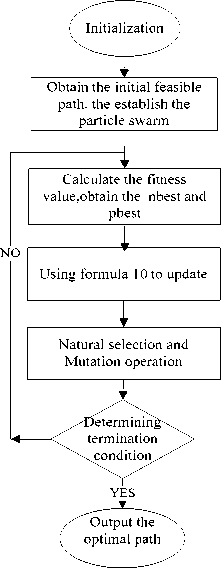
Fig. 2 Flow chart of the algorithm

Natural selection mechanism: The fitness values of the particles measure the strength of adaption of the particles, according to the fitness values we sort the particles and eliminate the weaker particles by eliminate probability.

Mutation mechanism: Using depth first search algorithm randomly to generates a new particle instead of the particle being eliminated by natural selection. The new one is thought as varying from the eliminated, so the history optimal solution and the neighbor’s optimal solution are saved.

The natural selection and mutation operations are after each round of updating in PSO algorithm.

• D.    Implemence of the algorithm

The flow chart of the algorithm is as Fig 2, and the steps of the algorithm are as follows:

• (1)    Initialization. Set the number of network nodes n , the network topology NET , link parameters matrixes, particles number N , maximum iterations M , the elimination probability P _c of natural selection and related values of the constraints: B-req, D-req, L-req, J-req;

(2)Generating the initial particles swarm x_i ( i=1,2…N ) by algorithm 1,when we know the source node s and the destination node d ;

(3)Calculating the fitness function value F(xi) of each particle by formula (9), determining the neighbor optimal particles G(t) and history optimal Pi (t) ;

(4)Updating each particle by formula (10);

(5)Natural selection and forced mutation operation;

(6)Judging the termination conditions, if satisfied, then to the step (7), if not then step (3);

(7)Calculating and outputting the global optimum, that is, the optimal path.

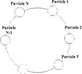
Fig.4 The second particle neighborhood selection approach

In this experiment we define two neighborhood selection approaches, the first one considers all the particles in the swarm as neighbors of each other, so the “nbest” is the “gbest”, the second one is connecting particle 1 and particle 50 in turn form a circle, each particle is the neighbor of each other if their number of the particle is near, as shown in Fig.4 We will compare the natural selection and mutation mechanism of the PSO algorithm to original PSO algorithm under the definition of the two neighborhood approaches, record each program by: 50GA-PSO, 3GA-PSO and 50PSO, 3PSO.

The experimental simulations are implemented by using the software of the Matlab.

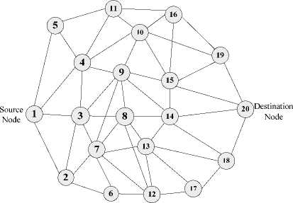
Fig.3: The network topology for simulation

The network topology is shown in Fig.3, which has 20 nodes and the number 1 node is source node, the number 20 is the destination node. From the network topology we can get the connection matrix: Net, which is a 0-1 matrix. If the node i and node j is directly connect, the i, j - th element of Net is 1, if the node i and j is not directly connect the ^{i ,}j - th element of Net is 0; the diagonal elements are defined as 0.

The values of the link parameters we can directly get from the network or predict from other layers of the network. In the experiment we generate them from the random matrix in a range. For example the bandwidth matrix B is an n*n matrix, the B ( i , j ) means the bandwidth parameters on link e ( i , j ) , the range of random values of parameters B are in the internal of [40, 60]. In the same way, we set the range of delay matrix D as:[0.5,1.5], packet loss rate matrix L as: [0.002,0.008] ， delay jitter matrix J as: [0.5,1.5],cost matrix C as:[2,8];and B_req=45,D_req=5,L_req=0.02, J_req=5; the number of the particle N =50; the parameters in fitness function: а=Р=ц= 1 , Y = 500 , the eliminate probability p c _{= 0} 4 ; The maximum number of iterations M =20. When all this parameters confirmed, we can obtain the fitness value of the optimal path is 18.

2      4      6     8     10     12    14     16     18    20

Iterations

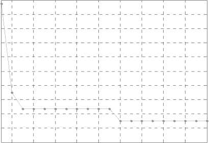
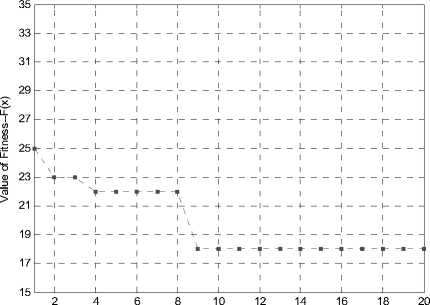
Fig.5 The fitness value changing process by 50GA-PSO

Fig.5 shows that the relationship between fitness function value and the number of iterations. Showing the progress of the 50GA-PSO algorithm find the optimal path under the network topology showed in Fig.3. At the first 11-th iterations, the 50GA-PSO cannot find the optimal path, however, at the 12-th iteration, the 50GA-PSO get the path whose fitness value is 18, which is the globe optimal path, so the 50GA-PSO algorithm is effective to solve the constraint routing problem. The convergence procedure of the path which is found by the 50PSO is shown as Table I

TABLE I.     the CONVERGENCE PROCEDURE OF 50 ga -PSO

Iterations	Path	F(X)
1	1-4-3-7-12-17-18-20	34.5147
2	1-4-9-14-20	22
3-11	1-3-9-14-20	19.7183
12-20	1-3-8-14-20	18

Fig.6 show the progress of the 3GA-PSO algorithm find the optimal path under the network showed in Fig.3. It tells us the relationship between fitness value and the number of iterations. And the Table II shown the convergence paths and their fitness values

Iterations

Fig.6 The fitness value changing process by 3GA-PSO

Iterations

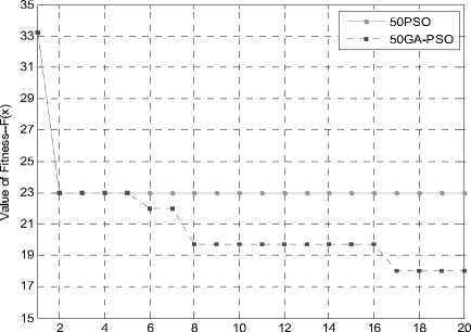
Fig.7 Comparisons of 50PSO and 50GA-PSO

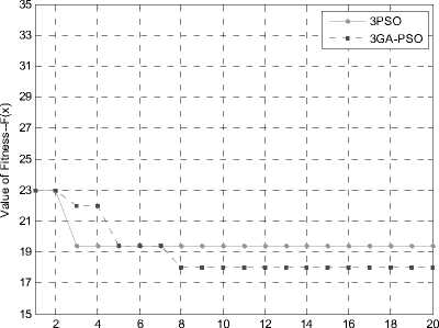
Fig.8 is the comparisons of 3PSO algorithm and 3GA-PSO algorithm. The 3PSO algorithm gets a better solution with the fitness value of nearly 19 at the third iteration, but it is a local optimal solution. The 3GA-PSO algorithm jump out of the local optimal solution for 3 times and at the eighth iteration it finally reaches the global optimal solution with fitness value of 18.

TABLE II.     the CONVERGENCE PROCEDURE OF 3GA-PSO

Iterations	Path	F(X)
1	1-2-3-8-13-17-18-20	43.1824
2-3	1-4-10-19-20	25
4-8	1-4-9-14-20	22
9-20	1-3-8-14-20	18

In the two figures above, we have seen that both the 50GA-PSO and the 3GA-PSO algorithm can get the path whose fitness value is 18, which is the globe optimal path. They are effective to solve the constraint routing problem. And then we will compare the proposed algorithm which with the ideas of natural selection and mutation mechanism to the original PSO algorithm.

As we can see in the Fig.7, the 50PSO algorithm falls into the local optimum, which no further changes after just gets a fitness value of 23. However, the 50GA-PSO jumps out of the local optimum and reaches the global optimal solution with the value of 18. It is because the 50GA-PSO algorithm has adding the natural selection and mutation mechanisms which makes the particles swarm diversified and the new particles increases new information in the process of searching a better solution. So the 50GA-PSO algorithm increases the probability to get the global optimal solution.

Iterations

Fig.8 Comparisons of 3PSO and 3GA-PSO

Fig.9 is the comparisons of 50GA-PSO and 3GA-PSO algorithm, both of them absorb the ideas of nature selection and mutation mechanism of the GA. the difference is the definition of the neighborhood selection approach. The 3 neighbors approach search a smaller range for a single particle but for the whole swarm they convey more information and search a lager range. As we can see in figure 9 ,both of the algorithms converge to the global optimal solution, but the 3GA-PSO converge faster to the global optimal solution; since the 50GA-PSO learning directly to the group optimal solution ,so it can get a sub-optimal solution faster than 3GA-PSO at the beginning of the search.

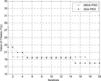
Fig. 9 Comparisons of 50GA-PSO and 3GA-PSO

For the optimization algorithms have the chance to fall into the local optimal solution and just get a sub-optimum, we define the search success rate to describe the effect of the algorithms. Search success rate is defined as the number of the experiments which find the global optimum solution divide by total number of experiments.

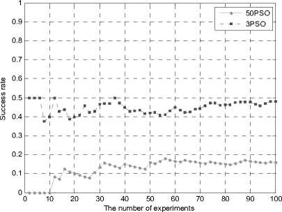
Fig.10 The success rate of 50PSO and 3PSO

The Fig10 is the search success rate of 3PSO and 50PSO compare by the experiment times, the Fig11 is the success rate of 3GA-PSO and 50GA-PSO compare by the experiment times, in Table III is the detail values searching success rate of the 50PSO, 3PSO, 50GA-PSO, 3GA-PSO algorithm at each experiments. From the figures and table we can see that in the first 20 experiments of 50PSO, the success rate is only 15%, after 100 experiments and the success rate is 20%, the 3PSO is a little better than 50PSO, but still not reach 50%, which means that the original PSO algorithm can easily fall into the local optimal solution, and it is hard to find the optimal path in the multi-constraints routing model. However, the 50GA-PSO has a much better performance than 50PSO, the success rate is 74% after 100 experiments and 3GA-PSO is even better, whose success rate reaches 85%. It is because the GA-PSO algorithms absorb the ideas of the nature selection and mutation mechanism of the GA and the particle swarms become diversified. In the progress of searching the optimal solution the GA-PSO algorithms increase the probability of jumping out of the local optimal solution and obtain the global optimal solution.

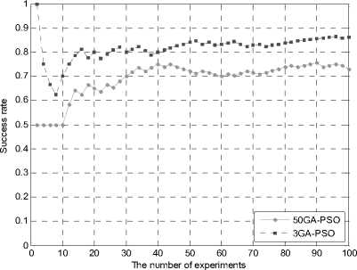
Fig.11 The searching success rate of 50GA-PSO and 3GA-PSO

TABLE III. the comparison of search success rate

Success rate	Experiment times
	20	40	60	80	100
50PSO	15%	15%	20%	18%	20%
3PSO	40%	45%	45%	49%	49%
50GA-PSO	65%	76%	70%	75%	74%
3GA-PSO	80%	80%	82%	81%	85%

• VI.  Conclusion

In order to meet the diverse needs of users on the network QoS, this paper provide a way to solve the problem. Firstly the multi-constrained QoS routing model was set up and the fitness function was constructed by transforming the QoS constraints to a penalty function. Secondly the iterative formula of PSO was improved so that it was applicable to the routing problem which is a non-continuous searching space. Finally, we introduced the natural selection and mutation ideas in the GA to the PSO to improve the performance of PSO algorithm, which made the particles more diversity. The simulation results proved that the proposed GA-PSO algorithms can not only successfully solve the multi-constrained QoS routing problem, but also achieve a better effect in the success rate of the search.

• [1]    Dorigo M, Birattari M, Stutzle, “Ant colony optimization” in: Computational Intelligence Magazine, IEEE Volume:1, Date: Nov. 2006. page(s): 28-39.

• [2]    M.K. Ali, F. Kamoun, “Neural networks for shortest path computation and routing in computer networks”,IEEE Trans. Neural Netw.1993, pp:941-954.

• [3]    Wen Liu,Lipo Wang, “Solving the Shortest Path Routing Problem Using Noisy Hopfield Neural Networks”, Communications and Mobile Computing, 2009. CMC '09. WRI International Conference, Jan. 2009, Volume: 2, pp: 299-302.

• [4]    Huang ShengZhong, Huang Liangyong. “The Optimal Routing Algorithm of Communication Networks Based on Neural Network”, in: Intelligent   Computation Technology and

  Automation (ICICTA), May 2010,Volume: 3, pp: 866–869.

• [5]    M. Munemoto, Y. Takai, Y. Sato, “A migration scheme for the genetic adaptive routing algorithm”, in: Proceedings of the IEEE International Conference on Systems, Man, and Cybernetics,1998, pp:2774-2779.

• [6]    C.W.Ahn,R.S.Ramakrishna,“A genetic algorithm for shortest path routing problem and the sizing of populations”, IEEE Trans. Evol. Comput.6, 2002,pp:566-579.

• [7]    Gelenbe.E, Liu.P, Laine J, “Genetic Algorithms for Route Discovery”, in:Systems Man and Cybernetics, PartB:Cybernetics,IEEE Trans, Date: Dec. 2006, Volume:36, pp: 1247-1254.

• [8]    G. Raidl, “A weighted coding in a genetic algorithm for the degree constrained minimum spanning tree problem”, in: Proceed- ings of the ACM Symposium on Applied Computing, 2000, pp:440–445.

• [9]    J. Kuri, N. Puech, M. Gagnaire, E. Dotaro, “Routing foreseeable light path demands using a tabu search meta-heuristic”, in: Proceedings of the IEEE Global Telecommunication Conference, 2003, pp:2803–2807.

• [10]    J. Kennedy, R.C. Eberhart, “Particle swarm optimization”, in: Proceedings of the IEEE International Conference on Neural Networks, 1995.

• [11]    Zhihui Zhan,Jun Zhang,“Adaptive Particle Swarm Optimization”, in: Systems,Man,and   Cybernetics,PartB:Cybernetics,    IEEE

  Transactions on Issue Date : Dec. 2009 Volume:39, Issue:6 pp:1362-1381.

She has been with the school of Information and Communication Engineering, Beijing

University of Posts and Telecommunications, since 2006, and is currently a Associate Professor. She is a reviewer of several journals. Her current research interests include subscriber traffics behavior and networks behavior analysis, future network architecture, routing, and resource management.

She has published over 30 papers since 2003 in the important journals / conferences, participated and edited two books, and applied eight patents.

Jian Li received the M.Sc. degree in next generation network from The Beijing University of Information and communication engeneering.

His current research interests include routing, and optimizing theoretics.