Performance Analysis and Enhancement of TCP in Presence of Jitter in Wireless Networks

Published Online June 2016 in MECS DOI: 10.5815/ijcnis.2016.06.02

Because of popularity in Internet services, current network traffic is dominated by the data generated by the applications such as web, email, multimedia downloads, file transfer, etc. [1]. One of the important affecting factors for providing QoS in wireless networks is packet losses. In wireless network, packet losses are due to congestion as well transmission. The congestion loss is due to burst traffic in the network and transmission loss is due to high bit error rate or jitter or frequent disconnections. Transmission loss occurs very frequently in wireless links which cannot be ignored. Packet loss due to transmission in wired links can be ignored [2], [3]. In addition to this, challenges for applying TCP over wireless link is an end-to-end congestion control. An end-to-end congestion control results in seamless data transportation. For a packet sent by the source, acknowledgement (ACK) is received before the timeout period. Otherwise this leads to a timeout loss and sender window (cwnd) size set to 1 packet. In this paper, we consider jitter which causes wireless transmission loss. Jitter is the variation in inter arrival time. Positive jitter value which is greater than half of the average round-trip value results in timeout loss. Any packet arriving after its scheduled time is discarded by the receiver. The problem of delay-jitter is thereby transformed into end-to-end delay and packet losses. Moreover, for a timeout loss, the sender TCP does an exponential backoff for some time. The effect of the backoff is that the window size does not grow for a small period, after which it starts growing at a normal rate. For timeout loss source reduces its sending rate which is unnecessary [4], [5], [6], [7], [20], [21]. Researcher tried to provide some solutions to these problems. Some of the proposed solutions by the researchers are Indirect TCP (I-TCP) Protocol [8], SNOOP protocol [9], Wireless-TCP [10], TCP Westwood [11], ACK pacing [12], ACK splitting [13] and so on. To recognise the loss is due to congestion or transmission, the researchers has proposed some schemes. Some techniques proposed to judge the loss events and improve TCPs throughput are [14], [15]. The problem with these proposed techniques is too difficult in implementation. To satisfy these problems for applying TCP over wireless link, we propose a scheme that can dynamically change the sending rate to the packet loss caused due to congestion or jitter. The model works on the principle of additive increase and multiplicative decrease (AIMD) to satisfy the properties of congestion control algorithm and also has the capability of distinguish the packet loss caused due to congestion or jitter. If the loss is due to congestion, congestion control algorithm is invoked and the loss is due to jitter, immediate-recovery algorithm is invoked. This makes sender window to recover from unnecessary reduction made at the source. To enhance the performance of TCP for further, we apply the stability analysis [16], [17], [18]. Conditions are obtained for asymptotic stability of wireless system using time-delay control theory. Using Hermit matrix method, a relationship between Pmax (RED controlling parameter) and β (jitter controlling parameter) is established. A stability boundary for Pmax and β is established in terms of wireless network resource parameters. Queue convergence analysis is made. An approximate solution for q(t) is derived. Models validation is made using Matlab. Result analysis is made using graphs and the statistical data.

• II.    Rate Based Jitter Estimation

The packet delay variation is called jitter. Jitter also can be an indicator of network health. Increasing jitter is an indication of increase in congestion and decreasing jitter is an indication of smoother transmission. This nature of jitter helps to distinguish the congestion loss and the transmission loss [19].

Let B_bi be the bottleneck bandwidth, S be the packet size, t₀^s and t₁^s be the time when the first and second packets are send one after the other from a source. Let t₀^d and t 1 ^d be the time when first and second packets are received at the destination. Without loss of generality, we can write B bn =S/(t 1 ^d - t 0 ^d).

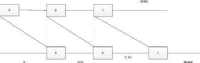
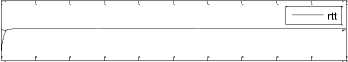
Fig.1. Time Diagram Showing Jitter

Let the receiver receives i^th packet at time t i ^d. But, t i ^d = t i ^s + tt i , where t i ^s is the time that i^th packet was sent, and tt i is the transmission time. The transmission time tt i = pt i (propagation delay) + q i (queuing delay at the router). In a single hop network where propagation time is same, pt i is almost same (constant). The queuing time, q i depends on (i) waiting time in the queue, and (ii) processing time which is very negligible. Under these assumptions, the difference between inter-reception time and inter sending time called Jitter. The inter-receipt time between two consecutive packets i-1 and i is denoted by irt_i.

irt i = t i ^d – t i-1 ^d = (t i ^s + tt i ) – (t i-1 ^s + tt i-1 ) = ( t i ^s – t i-1 ^s) + (tt i – tt_i-1)

irt i = ( t i ^s – t i-1 ^s) + ((pt i + q i ) – (pt i-1 + q i-1 ))

irt i = ( t i ^s – t i-1 ^s) + (pt i – pt i-1) + (q i - q i-1 )

In single hop network propagation time is constant. This implies that pti is constant. Thus

(pti – pti-1) → 0. Also, the sending timings of the packets, tis and ti-1s are known entities. Hence, the only variant is the queuing time. Therefore, jitter is the varying queuing time measured at the destination. Jitteri = qi – qi-1. The occurrence of jitter can be noticed by measuring the variation in queuing-delays at the destination. Jitter can be positive, negative, or zero. This leads to the following conclusions. (i) When variation in queuing-delay is positive then ith packet gets more delayed than the (i-1) th packet, (ii) Variation is negative then the ith packet reach destination in less time than (i-1) th packet, and (iii) variation zero indicates that the network congestion remains unchanged over the time scale of consecutive packets. We are interested in (i). The later packet reaches the destination taking more time than the previous packet, causing positive delay-variation in the inter arrival time. This is due to transmission error and in wireless networks this occurs in more frequent. The positive delay-variation in the inter arrival time results jittering and triggers into timeout loss.

• A.    K/W Transmission loss-predictor

Let L t (t) be the wireless transmission loss occurrence after the first packet transferred and ACK has received by the source. Source TCP check whether the jitter-loss is greater than the value of k/w or not, where k is a control parameter and w is the current window size. The ratio k/w indicates that k packets are in the queue at the router when TCP injects w packets into the network. Since TCP adds one packet per RTT, 0 < k ≤ 1. Using the scheme proposed in [2], K/W loss-predictor, distinguish the packet losses as follows. (i) The next packet loss is due to congestion when, (a) the source receives triple-duplicate acknowledgement, (b) the arrival of ACK is longer than one RTT (Next-RTT), and Jitter value is greater than k/w value. (ii) the next packet loss is due to transmission when, the arrival of ACK is longer than one RTT (Next-RTT), and Jitter value is less than or equal to k/w.

• B.    Pseudo-code for loss identification

jitter i = q i – q i-1

if (next-rtt >0 and jitter i > k/w), \ congestion loss

β = 0, \ Invoke congestion control algorithm end if ( next-rtt >0 and jitteri ≤ k/w) \ Transmission loss

β > 0, \timeout-loss, invoke immediate-recovery algorithm end

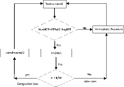
Fig.2. TCP Loss Prediction and Recovery Flow Diagram

When loss is due to congestion, the jitter control parameter, β =0. The threshold value of sender window is fixed to half of the current window size, and slow start phase started. When the loss is due to transmission because of jitter, the sender TCP has experienced it as timeout-loss and decreases the window size to 1 which is unnecessary. To recover from this loss the system invoke immediate-recovery module. The recovery rate is proportional to β times the flow rate of the previous rtt.

• III.    System Model for Wireless Networks

The extended fluid model [19, 20, 21] that describe the dynamics of the TCP congestion window size in wireless networks in presence of jitter is, dW(t) =    -α W(t) La(t) +β Lt(t)     (1)

TCP operates on AIMD congestion control strategy. The factor α is decrease rate of source window which is considered as 0.5, L a (t) is the arrival rate of packet losses due to congestion at time t and L_a(t) =   ^{(   ( ))} p(t-

R(t - R(t)) ). This loss is proportional to the throughput at the source. First term on the right hand side of equation (1) refers to linear increase of the sender window size until congestion occurs at the destination. The second term refers to congestion control based on the feedback received from the RED router. The third term L t (t) refers to immediate-recovery due to jitter loss. The jitter loss is proportional to the sending rate of the source. Therefore, L t (t) is proportional to ⁽ ^ ⁽ .

The equation (1) can be modified to,

_{=    -}   ( ^ ) (t-R⁽ t ⁾⁾ p(t-R(t))+β ( t~R⁽ ^ ⁾⁾   (2)

St =  ( ; )-  2R(t-R( )) p(t-R(t)) +βR(t-R( ))  (2)

β is jitter loss control parameter and by choice β ϵ[0,1]. The dynamic behaviour of instantaneous queue length is given by dq(t)_ N w(t)

St      R(t) - Cd                  (3)

Where, w(t)/R(t) is increase in queue length due to sending rate of the packets by N- TCP flows. C d = q(t)/R(t) is the decrease in queue length due to servicing of packets and delay due to packet departure from the router. The mathematical version which represents packet dropping probability of RED is given by

0 ,               q(t) ∈ [0, t_min]

P(t) =  W⁽⁾^ P_max , q(t) ∈ [t_min, W_max]   (4)

⎪ max min

⎩   1 ,            q(t) ≥ W_max

Congestion loss is assumed to happen when queue buffer of the router reaches a value of Wmax packets. The maximum buffer size, Wmax of the router is calculated by, Wmax = R(t) +M , Where Cd /S is the bandwidthdelay product, M (in packets) is the maximum buffer size of the router and R(t) is the round trip time. The buffer overflow takes place when the queue length becomes larger than Wmax value. Cd is the down-link bandwidth. The model describing round trip time (RTT) in wireless networks is given by, R(t) = ( )+Tp , Tp is the propagation delay in the wireless media, q(t)/Cd models the queuing delay.

• IV.    Time-Delay Feedback Control System

In this section, we study the stability analysis of TCP in presence of jitter in wireless network system. The procedure applied is as follows: First linearize the system models, using Hermite matrix for time-delay control system, explicit condition under which the system is asymptotically stability is derived. A relationship for P max and β is obtained. Mathematical relations are derived for stability boundary of RED control parameter P_max and jitter control parameter β in terms of network resource parameters. Convergence analysis of queue length in presence of jitter is discussed.

• A.    Linear Model Derivation

Let x(t) be a general non-linear function defined by, x(t) =f(u(t), v(t), t) , where, u(t) represents the sender window dynamics, and v(t) represent the queue dynamics at the bottleneck link. We assuming that f(u(t), v(t), t) has smooth and continuous derivatives around the equilibrium point, Q₀=(w₀, R₀, q₀, p₀) . Using Taylor’s series expansion, the linear function of nonlinear function, ignoring second and higher order partial derivatives is,

f(u(t), v(t), t) = f(u0(t), v0(t), t0) + fu(t)δu(t) +fv(t) δv(t) +O(δu(t), δv(t))

where f_u(t) = £ |(u₀, v₀) , f_v(t) = £ |(u₀, v₀) . The linear models of the equations (2) to (4) are derived around the equilibrium point Q ₀=(w₀, R₀, q₀, p₀) . Let N be the number of TCP flows. At Q 0 , the steady state conditions of equations (2) and (3) are given by, ẇ(t) = 0,q̇(t)=0 .

The estimation algorithm is based on small signal behaviour dynamics, therefore, at the equilibrium point, without loss of generality, we can assume,

w(t) =w(t-R(t)) =w₀, q(t) =q(t-R(t)) =q₀, p(t) =p(t-R(t)) =p₀, R(t) =R(t-R(t)) =R₀           (₅)

Using equations (5) in ẇ(t)=0, q̇(t)=0, and after simplification we get, p0

2 0Wq+2 W_O²

|sI-А-Ее ^R₀S|=0            (13)

Let, w_R=w(t-R(t)), p_R=p(t-R(t)) . From (2) we get,

u(w, w_R, q, p_R) = 5 (;₎ - ⁽ I ⁾ 5 ( ) ⁽ - ⁾ p(t-R(t))

+β                        (6)

()

To linearize equation (6), find all the partial derivatives of u(w, wR, q, pR) with respect to the variables at the equilibrium point and defining,

δw(t) =w(t) -w0, δq(t) =q(t) -q0, δp(t) =p(t) -p0

After simplification, s²+(— +     + —)s+

V^R₀ R_o C_d Rq/

(%+

4 R0 Cd

e -Ros)=0

2NB /

The characteristic equation (14) determines the stability of the closed-loop time-delay wireless system in terms of the state variables 5 w(t) and δq(t) .

• B.    Stability Analysis

Denote, P(s, e ^R₀S)= s²+

(₽ +    + ^-)s+( \+ -^ +   e R0S )

^R0 Ro ^d R0 ^R0 R0 ^d 2NB /

δẇ(t) =ẇ(t) -w0, δq̇(t)=q̇(t)-q0

δp(t) =  (q(t) - t_min) - p_{0 ,} where B= W_max – t_min,

L= pmax

δẇ(t)=-( £ + Ro2 Cd )δw-     δpR

δq̇(t)=г δw(t) - г δq(t)

Ro

δp(t-R0) = 5 (δq(t-R0)) + 5 (q0-tmin) -p0

Using equation (9) in (7), we get

δẇ(t)=-(^ + R02cd ) δw(t) - ^δq(t-R0) +

Let e -ROS=z,and a0=1,a1=  + ^ +,

,           0       ,1

_ P a2=  2+     +e

P(s, z) =a0 s2+a1 s+a2

The Hermit matrix for time-delay control system of equation (15) is

(0,1)(0,2)

H = [(0,2)  (1,2)]

(0,1) = 2a₀a₁ = ²- ⁽ j^l ) ₊

(0,2) = -2a2 Im(z) = -^ Im(z)

^LCd^2R0 (t -q)+ ^Rn^cd²Pn ^{min 0}

(1,2) = 2a1Re(a2) =

Denote, x(t) =[ ^w()] , then

2( 3+  22N  +   )( ₽2 +  23N  +)

RO RO Cd RO RO RO Cd 2NB

Put V     p - -IL 1 v - LCd2

Put, x1=   +     + ,x2=,

,12

Where,

ẋ(t) =Ax(t) +Ex(t-R(t)) +F

^ +

-( ₽ + ^)

A= (       )

=

0₀ "^LRo^cd² 1 ] E=[⁰₀   ²₀  ],

R0J

F =[ 2N^ZB ^(tmin

-q0)+ °2N2 °]

Solving linear differential equation (11) using Laplace transform technique with

L{x(t)} = x(s), we get

(ѕӀ-А-Ее-^R₀S ) x(s) =           (12)

Let      z=ei“, z=cοsω+isinω, Re(z) = cοsω,

Im(z) = sinω , then

2x

H(e iM) =[-x2sinω

-x2 sinω 2x1(x3 + cοsω)

• C.    Stability Conditions

The time-delayed control system (2) to (4) is asymptotically stable in terms of stable variables δw(t) and δq(t), iff the following two conditions are satisfied.

Condition1: The Hermit matrix H(1) = H(e io ) is positive.

The characteristic equation of (12) is,

2x        0

H(1) =[ ₀¹  _2x1(x3+ ч )]

0<β<(Pmax£rL^oE + 2N )

V 2NB ROcd^

From the determinant, 4x₁² (x₃ + ^2)>0 , after simplification,

=-     ^4N2B A

L=pmax> -(Ro^Cd^ +)

β>-(Bmax^idEjlf)2 +)

β()

Condition 2: For all ωϵ[0,2π], detH(eio)>0, leads to the following inequality.

V. Convergence Analysis of Dynamic Queue

In this section, we discuss the convergence of buffer queue in the router. From equation (12),

(s I – А – Е e -ROS)-1=    \  [y1y2

V                    2         p( ,e Ros) y3y

Where, У1=s+  ,У2=- 2N^B 0 ,У3=,

₌ p

У = ++

Equation (13) can be written as

(2x1) (2x1 (x3 + 2 ))

cοsω

-x22sin2ω>0

x(s) =

H(e 1Ш ) = x22cοs2ω + 2x12x2cοsω +

F s p(s, e -ROs

[y1

) y3

y2

y4

4x12x3-x22>0

After simplification, X (s)

У5 sp(e ^Ro

) [^yy1₃] ,

The necessary condition for (16) to be true is the discriminate, Δ>0

or [^δδ^WQ(⁽s^s)⁾] =y5 [^yy1₃]             (21)

_ -x12 ±√xT2 (xV'-ZxZ)+x22 cοsω= x2

Where,

By the properties of cosine function, for ωϵ[0,2π], cοsω ϵ[-1, 1]

The conditions can be written as,

^y 5 ⁼

LR0cd

2( t„_in-q ⁾ R C_d²p_i

2NB

2N'

S p(s,e"Ros)

From equation (21),

x12 √ EZ ( x^^EZE ) ^2 >1

√ EZ ( ЕЕЕЕЕЕз ) +EZ < -1

By direct manipulation, there is no solution for the inequality (17). From (18), we obtain

П           f 20NB 4N²B

0<      < (      +      )

0<β<(Ртах cd2 R02 + /r )(20)

p V 2NB       Ro Cd/

(

5Q(s) =    ⁽

δQ(s) =

δQ(s) = s2 + T

(

b^d! (Qn) +^o£d^Po (             )               )

sP(s,e"Ros)

( 2N )( ^{( t}min Qp ⁾ +Pp ⁾

sp(s,e"Ros)

1C 2 L

( ( '-min Чр) +Pp)

c4-( P , 2N )    (

e Ros

D. Theorem 1

Given the wireless network parameters Cd (down link capacity), Cu (up-link capacity), N (number of TCP sessions), R0 round-trip time, and B RED control parameter, the wireless network system given by (2) to (4) is asymptotically stable in terms of the state variables δw(t) and δq(t) if and only if the control parameters Pmax and β satisfies

δQ(s) = ^TTTT^TsZ^rT^      (23)

s^+x1 s+x3+^e Kos

Where, _y6=      ( ( t_min-q₀) +p₀)

П / n       f 20NB

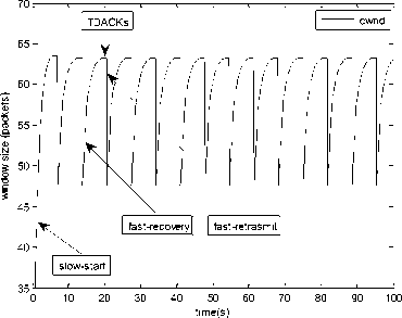
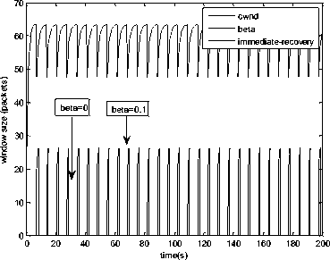
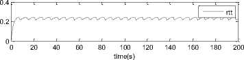
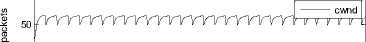
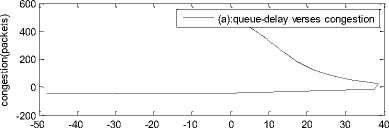
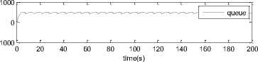
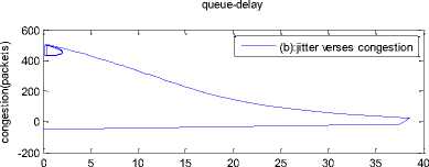
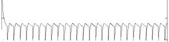
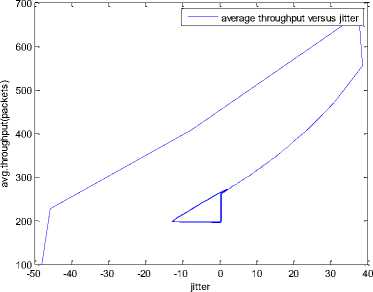
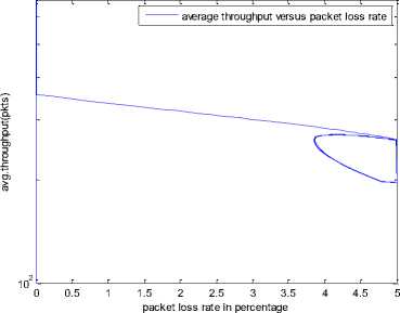
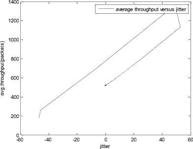
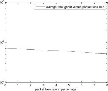
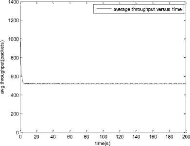
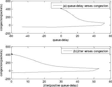
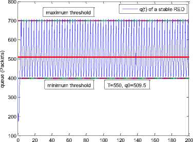
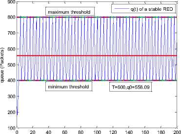
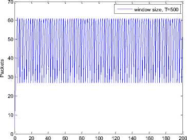
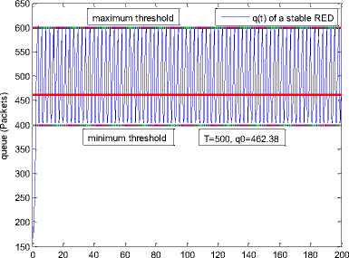
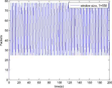
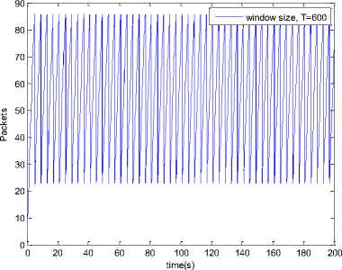
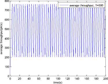
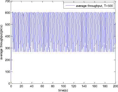
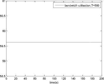
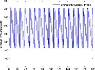
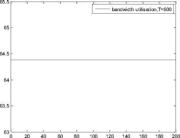
0

_max< (

XK0 Ld

+ 4N2B )

+      )

R0 cd 7

A. theorem 2

Given the wireless network parameters Cd, Cu, N, R0 and B, on the basis of wireless network system given in (2) to (4), an approximate solution of q(t) is pxt        yt 1

q(t) =q +y [     -     +  ]

(x-y)(x-y) У  xy

If the RED control parameter Pmax and jitter control parameter β satisfies

⁰

max^≤zkt√

0<β≤    √A₂²-4 A₁ A₃

P —       2Ad

Where ξi‘s and Ai ‘s are given in (28).

Proof: Expanding e-R0s, using Taylor’s theorem about the stability point discarding the terms of order three and higher, e -R0s =1-R0s+

From (23), S²+x₁s+x₃+2z e ^RO^S . This simplifies to

.        4N 2 2LC ,2

А2=—- — -

Д =      4N24N

А3=   +R ,

(LCd2Ro)2--

V 2NB / NB RQB

Solving (26) for L=Pmax and (27) for β, we get

0

0<β≤Az+ √A^^4A^^(30)

From Equation (23)

s2+(3+ 22N + ^-)s+ kR0 R02Cd Ro/

δQ(s) =

_______Уд_______

(л_гs²+r₂ 5+л₃ )

( ₽2 +

R0 R0 Ld

]p 2               p 2„2

+    (1-R0+    ))

δQ(s) =

____Уд____

(   )(s-y)

( 1+

1^i!Sl)s²+ 4NB / *

'³_{+     +   -}LRqC^'

q R₀²C_dRq 2NB ,

Using partial fraction,

+( %+ 23N +

\Rq R_o C_d 2NB

δQ(s) = y6[

1      1

(x-y)(   )

-

-   +]

у(x-y) s—у   xy s

Put и1=(1+LR^) ,η2= 3+ -4 +  - LRqC^ ,

1               ,2,

В , 2N , LC ,2

η3=+—3 +

η1 s2+η2 s+η3

If Δ>0, equation (24) has distinct roots given by x,y= ±√(25)

where, x takes + and y takes – of ±.

The discriminate of (25) is positive. After simplification for the discriminant, and expressing in terms of L and β, we get,

ξ1 L²+ξ2 L+ξ3>0        (26)

А₁β²+А₂β+А₃>0        (27)

where,

Taking Laplace transform, г pxt pyt 1 1

δq(t) =y6* (X-y)-у(X-y)+xy +

q(t)=q₀+y₆*(X-y)^-у(X-y)⁺xy +      (31)

B. theorem 3

Given the wireless network parameters Cd, Cu, N, R₀ and B, the instantaneous queue length converges to the target, T=⁽^"mi"n^"^WTnnx⁾if and only if RED control parameter, P_max and jitter control parameter β satisfies

Pmax=K1 K2+K3

β=K4 K5

where Ki’s are given by (35).

Proof: From equation (23), lim t→ oo ^Q (t)=lims→osQ(s)=

ξ2

ξ1= (Sl^)2 1

Zpc^ +   +

NB R0B NB

lim_s→

0 s2+x1 s+x3+^e Ros limt→ OO SQ (t)=lim s →osQ(s)=       +q0

/ limt→   (t)=q0+limt→ oo ^Q (t)

limt→mq(t)=q0+x3+—

Let lim q(t)=^min + wmax t→

Then

Pmax=K1 K2+K3

β=K4 K5

Where

К =

K1=+

K0 Ld K0 Ld

K2=2q0-tmin-wmax

К _ _4pN_4N

K3=+

K0Ld K0 Ld

K=^Pmax^RO^2cd²~^4N2

K5=1+   (2q0 - tmin - wmax)

K0Ld

Theorem 3 gives a relationship between Pmax , β and q0. The relations given in (33), (34) and (35) not only leads to the stability of the system but also brings the instantaneous queue length to converge to the given target value.

• C.    theorem 4

The wireless network system (2) to (4) is asymptotically stable in terms of the state variable δw(t), δq(t), if the equilibrium value of the queue level q0 satisfies bninj2^max -     

• -    -  + √ξ₆

Proof: Using (33) in (29)

01 K₂+K₃≤321√

Substituting for K1, K2 and K3 from (35), and simplifying for q0, we get --   

ξ₆=^4[(2β+1+-^-)²+

• ⁶ V Ro^d^

(β-1)2+ГГ ( ГГ-β-1)]

R^O^d ^Ro^d '

2N

^ξ7⁼    (β+     )           (37)

c 2 ξ8=

Theorem 4 gives a stable value for q0. With help of this value one can tune the network system parameters to achieve queue convergence and hence obtain good throughput.

• VI.    Simulation and Performance Analysis

  
  
  

  Wired Link

  
  
  
  
  
  

  Wireless Link

  

  Destination

  
  

  Source                  R1

  
  

Fig.3. Network Model

A number of simulation experiments are conducted using Matlab R2009b to evaluate the performance of TCP. Fig.3 shows a typical network topology of a heterogeneous network. R1 and R2 are the routers and the TCP which has been modeled represents the last hop transmission between R2 and destination. The propagation time is assumed to be 50 ms. The bottleneck bandwidth (Cd) is 10 Mbps, packet size is 1000 bytes and load factor is 10 TCP sessions, k=1, R0=0.1s.

• A. Experiment1: Un-stable network system

Fig.4. Slow-Start, Congestion Control and Recovery

Fig.5. Cwnd Recovery due to Jitter-Loss

0    20    40    60    80    100   120   140   160   180   200

time(s)

packets

Fig.6. Performance of rtt, cwnd and Queue w.r.t Time

jitter(positive queue-delay)

Fig.10. (a) Congestion due to Queue-Delay (b) Congestion due to Jitter

\        average throughput versus time

0    20    40    60    80    100   120   140   160   180   200

time(s)

Fig.7. Performance of Throughput w.r.t Time

Fig.8. Variation of Throughput w.r.t Jitter

Fig.9. Performance of Throughput w.r.t pkt. Loss

The trace of the graph of fig.4 represents the typical behaviour of cwnd. The slow-start phase initiate data flow over the connection and increases continuously for every rtt until loss occurs. When the sender cwnd reaches a maximum size of 64 packets, buffer in the bottleneck router starts overflowing. The source receives TDAKs, the cwnd is reduced to half of its current value. For a timeout loss the window size reduces to 1 packet. In addition to timeout loss, the sender does an exponential backoff for some time. The effect of backoff is that the window size does not grow for a small period, after which it starts growing in the normal rate.

To add intelligence to TCP that packet loss is due to transmission and not due to congestion, and mitigate backoff loss, we introduce the term Lt(t) in equation (2). The traces in fig.5 represent immediate-recovery of sender window due to jittering. The timeout loss experienced by the source and reduction made in its sending rate is unnecessary. To recover the loss TCP initiates immediate-recovery algorithm. The amount of recovery is proportional to sending rate in the previous RTT. The jitter value is compared with k/w value. If it is congestion loss then β =0, congestion control algorithm is invoked. If it is jitter loss then β=0.1. The traces of fig. 6 represent that the queue length oscillates with the sender window and similarly RTT varies with queue length. As the sender window increases, the queue length also increase because the sending rate by the source is higher than the service rate by the bottleneck router. The bottleneck bandwidth considered is 10 Mb/s. When the cwnd reaches 44 packets then the queue length reaches a minimum threshold value of 200 packets. We observe that when the cwnd is between 45-64 packets, number of packets in the queue is higher than 200 and the congestion avoidance event starts. The bottleneck router stars dropping the packets randomly. Sender TCP on receiving TDACKs, halves its cwnd size.

Throughput depends on the source sending rate. The graph of fig.7 shows that throughput varies over the range of 200 to 280 packets corresponding to cwnd 47 and 64 packets respectively. The traces of fig. 8 show the behaviour of throughput with respect to jitter. In the beginning of the simulation, jitter value is negative resulting highest throughput. As the simulation time lapses jitter value becomes positive resulting in the

decrease of throughput. When the jitter value reaches a maximum of 40 ms throughput drops suddenly to a small value. Traces of fig. 9 represent that throughput decreases with the increase of percentage packet loss rate. When the loss rate is between 4% to 5%, throughput falls by 30% but recovers immediately. The occurrence of jitter can be noticed by measuring the variation in queuing-delay at the destination. fig. 10(a) represents the variation of congestion in the bottleneck router with respect to (w.r.t) queue-delay. The later packet reaches the destination taking more time than the previous packet, causing variation in the inter arrival time of packets. This is due to transmission and is more frequent in wireless networks. Thus, Jittering triggers into timeout loss. fig. 10(b) gives the traces of congestion with respect to jitter. From the graph, the congestion slowly builds up with respect to increase in jitter, when jitter decrease, congestion reaches a maximum value of 500 packets because of the fact that many TCPs sessions are pumping large number of packet into the network (load), resources are being shared optimally.

B. Experiment 2: Stable network system

Fig.13. Stable Throughput w.r.t Jitter

0.4

0.2

cwnd

0     20    40    60    80    100   120   140   160   180   200

time(s)

Fig.14. Stable Throughput w.r.t pkt-loss

0     20    40    60    80    100   120   140   160   180   200

time(s)

queue

-500

0     20    40    60    80    100   120   140   160   180   200

time(s)

Fig.11. Asymptotic Stability of rtt, cwnd, Queue

Fig.12. Stable Throughput

Fig.15. (a) Stable Congestion due to Queue-Delay (b) Stable Congestion due to Jitter

Fig. 11 to fig. 15 are the graphs of stable network system. The experiment was conducted by assuming the propagation delay as 50 ms. The bottleneck bandwidth is 10 Mbps, packet size is 1000 bytes and load factor is 10 TCP sessions. Minimum and maximum threshold values of the queue buffer are 200 and 500 packets respectively. The initial values of R0=0.04s and β=0 and using relation (19), initial value of pmax was calculated. Using this initial pmax value and relation (20), next value of β was calculated. After small laps of simulation time, P and β converges to values 0.1067 and 0.3846 respectively. Traces of fig. 10 and fig. 11 shows that rtt, sender window size, queue length and throughput values stabilise to 0.21s, 56 packets, 425 packets and 520

packets respectively. The graph of fig. 13, fig.14 and fig.15 gives the variation of throughput with respect to jitter, variation of throughput with respect to packet-loss rate and variation of congestion with respect to jitter respectively. The graphs are smooth and not oscillatory. The experimental results shows that for a given resources, stability boundary increases the throughput value by 30% by minimising the packet losses.

• C. Experiment 3: Queue convergence analysis

  The simulation was conducted for different target values as summarised in table 1. For each of the simulations, the stability range of q0 was calculated using relation (36), Using the q0 value, Pmax value was calculated using relation (29) with an initial value of β=0.1, and finally using the value of pmax, β was estimated using relation (30). In simulation 1, target queue length, T=500, the range of q0 is (459.8, 464.96), chose q0 = 462.38, Value of P_max =0.544, and β=0.0089. The graph of instantaneous queue length is as illustrated in fig. 4.16. Approximately, 93 % of the traces of the graph values fall around q₀. In simulation 2, target queue length, T=550, the range of q₀ is (506.32, 512.69), chose q0 = 509.5, Value of Pmax =0.0013, and β=0.0024.The graph of instantaneous queue length is as illustrated in fig. 17. About 96 % of the traces of the graph values fall around q0. In simulation 3, target queue length, T=600, the range of q0 is (555.16, 561.03), chose q0 = 558.09, Value of Pmax =0.112, and β=0.0018. The graph of instantaneous queue length is as illustrated in fig.18. Almost, 93 % of the traces of the graph values fall around q0.

Table 1. Simulation results

1	2	3	4	5	6	7
1	(400, 600)	500	(459.8 ,464.96)	462.38	0.544	0.0089
2	(400, 700)	550	(506.32, 512.69)	509.5	0.0013	0.0024
3	(400, 800)	600	(555.16, 561.03)	558.09	0.112	0.0018

1: Simulation, 2: Minimum and Maximum threshold, 3: Target queue, 4: Stability range, 5: q0- value, 6: Pmax -value, 7: β-value.

time(s)

Fig.17. Queue Length when T= 550 Packets

time(s)

Fig.18. Queue Length when T= 600 Packets

time(s)

Fig.19. TCP Window when T= 500 Packets

time(s)

Fig.16. Queue Length when T= 500 Packets

Fig.20. TCP Window when T= 550 Packets

Fig.21. TCP Window when T= 600 Packets

Fig.24. Average Throughput when T= 600 Packets

Figs. 19, 20, and 21, illustrates the traces of TCP window dynamics for the threshold values 500, 550 and 600 respectively. Cwnd varies over the range (26, 60), (24, 77), and (22, 85) for T=500, 550, and 600 respectively. As the value of T increases, the lower bound of decreases whereas upper bound increases.

Fig.22. Average Throughput when T= 500 Packets

Fig.25. Bandwidth Utilisation when T= 500 Packets

time(s)

Fig.23. Average Throughput when T= 550 Packets

0    20    40    60    80    100   120   140   160   180   200

time(s)

Fig.26. Bandwidth Utilisation when T= 550 Packets

time(s)

Fig.27. Bandwidth Utilisation when T= 600 Packets

Figs. 22, 23, and 24 illustrate the traces of average throughput and Figures 25, 26, and 27 illustrates the traces of bandwidth utilisation for different threshold values. The bandwidth utilisation increases with the increase of target values.

• VII.    Conclusion

In this paper, we enhance the performance of TCP in presence of jitter in wireless networks. Jitter is one transmission loss which occurs most frequently in wireless networks. Jitter leads to timeout loss resulting sudden drop in the throughput. The model has the capability of recognising the congestion loss from that of jitter loss. k/w loss-predictor technique is used to achieve this task. k/w loss-predictor function uses queuing-delay and average rtt-delay (Next-RTT) as an input for prediction. When the sender TCP identified that next packet loss is due to jitter, the loss incurred in the throughput is tried to recover using immediate-recovery algorithm considering β=0.1. The proposed model also provides an end-to-end congestion control. For further improvement in the performance of the model, we discuss stability analysis. A time-delay control theory is applied. The application of asymptotic stability helps in tuning the control parameters pmax and β so that the network system works in a stable condition. This also controls the oscillatory behaviour of the RED router. The implementation minimises the packet loss and increases the throughput approximately by 25%. In the last section of the paper, convergence analysis of queue length is discussed. An approximate solution for q(t) is derived. Convergence of q(t) for a given target value subject to that pmax and β satisfies certain condition is established. The stability region of q0 is also presented there by our results provide global stability and convergence condition of the system. The described model works for networks which are associated with queuing servers with constant or variable service times. The model presented in the work is efficient, fair and adaptable to wireless networks.