Performance Analysis for Detection and Location of Human Faces in Digital Image With Different Color Spaces for Different Image Formats

Published Online July 2012 in MECS                                       and Computer Science

The face detection problem is to identify and locate a human face in an image [11]. The problem has important applications to automated security systems, lip readers, indexing and retrieval of video images, video conferencing with improved visual sensation, and artificial intelligence. Many different techniques have been developed to address this problem. Most methods are content-based. That is, they detect faces by attempting to extract and identify key features of the human face. Yow and Cipolla developed a method that elongates the image in the horizontal direction and identifies thin horizontal features, such as the eyes and mouth, using second-derivative Gaussian filters [1]. A technique developed by Cootes and Taylor matches features to a model face using statistical methods [2]. Leung, Burl, and Perona presented a similar method that matches features to a model face, except they used a graph-matching algorithm to compare detected features to the model [3]. Rowley, Bluja, and Kanade developed a front-view face detection system that feeds small 10x10 pixel images into a neural network [4]. Instead of using neural networks, Sung and Poggio developed an example-based learning method [5] while Colmenzrez and Huang used a probabilistic visual learning system [6]. A survey of content-based techniques for general image retrieval can be found in [7]. Unfortunately, contentbased techniques are very complex and expensive computationally. This is because it is difficult to develop techniques that are scale and rotation invariant. Also, if the face is rotated or partially obscured, the technique has to incorporate other techniques to solve the image registration and occlusion problems. In addition, it is often difficult to adapt the methods to color images. Color-based techniques [12] calculate histograms of the color values and then develop a chroma chart to identify the probability that a particular range of pixel values represent human flesh. The implementation of colorbased techniques is fairly simple and, after the system has learned a chroma chart, the processing is very efficient. Also, the methods handle color images in a more straightforward manner than the content-based methods. However, as [8] describes, color-based techniques have several drawbacks. Specifically, these disadvantages as written by Androustos et.al. is: “Histograms require quantization to reduce the dimensionality”. “The color space which is a histogram can have a profound effect on the retrieval results”. “Color exclusion is difficult using histogram techniques”. “Histograms can provide erroneous retrieval results in the presence of gamma nonlinearity”. “The histogram captures global color activity; no spatial information is available”. This paper will address the drawbacks presented above. First, quantization will necessarily lead to the loss of color information and an increased number of bins require an increased storage space. But if the number of bins is chosen judiciously, a color-method can strike a balance between storage space and accuracy. Second, the choice of color space for a particular method can be made by testing the method under different color spaces. There is debate over which color space is most appropriate for detecting human skin tones. Chroma charts have been developed for the standard RGB color space [9], the YIQ color space [10], the HSV color space [11,12], and the LUV space [13]. Third, color exclusion can be achieved by carefully omitting certain bins from the histograms. Fourth, one can make a color-based method more robust in the face of gamma nonlinearity by preparing the chroma chart for skin tones under several different gamma values. It should be noted that content-based techniques also have difficulty in the presence of gamma nonlinearity, because edge detection is more difficult for very bright or dark images. The fifth drawback is the most significant. Without spatial information, a colorbased method detects the presence of human flesh, not necessarily human faces. That is, a method based solely on color information would be unable to tell a face from a foot. However, many applications try to identify the presence of people in images, so the detection of flesh tones is sufficient. The lack of spatial information can also be viewed as an advantage, since color-based methods are less sensitive to object rotation, image rotation and scaling, and occlusion. That is, a color-based method is by design scale and rotation invariant. It should be noted that since flesh tones are very unique, colorbased methods are appropriate for face detection, but the methods do not generalize to detection of arbitrary objects.

The detection of human face in digital image has been made by Todd Wittman ([15]-[16]). He had successfully separated the images containing the face and images which are non face. Non- face means the images which has no human face. In his paper [15], he had used Levenberg–Marquardt training algorithm to detect whether the human face is present in a digital image or not. But the position of face inside the image has not been indicated. In his next paper [16], he had used image segmentation technique to localize the face position. This procedure did not work successfully. In this paper, the proposed algorithm has tried to make up the draw back of the technique which has been used by Todd Wittman [16]. The algorithm is very simple. First, it trains the network by Levenberg –Marquardt training algorithm so that it can detect face or non faced image. Now the threshold value of the network above which is a face and below which is a non-face is determined with the network output graph and is different for different color spaces for each of the image formats bmp, jpeg, gif, tiff and png. This depends on the training of the network. The algorithm takes an input image and chooses initial windows of size 300x300 which scan the whole image and take the mug shot each time and feed it to the neural network trained earlier with Levenberg –Marquardt training algorithm. If the output is greater than the threshold value, then it is a face described by a square drawn on it. The same operation is performed with reduced window size, diminished by 50 and continued till the size becomes 100x100. So all faces between size

300x300 and 100x100 will be detected. If there is redundancy i.e., two or more squares of different sizes represent the same face, then the squares of smaller sizes are omitted. This simple approach has not been made earlier and also a comparison with six different color spaces has been done to choose the appropriate color space. This is the reason for making this paper.

The proposed algorithm is run for each of the six color spaces RGB, YES, YUV, YCbCr, YIQ and CMY for each of the image formats bmp, jpeg, gif, tiff and png. The different image formats may affect the performance and accuracy of detection and location of human faces in a digital image of a particular image format. The different image formats are described below.

• A.    BMP (Bitmap)

BMP files are an historic (but still commonly used) file format for the operating system called "Windows". BMP images can range from black and white (1 bit per pixel) up to 24 bit color (16.7 million colors). The first part is a header, this is followed by an information section, if the image is indexed color then the palette follows, and last of all is the pixel data. Information such as the image width and height, the type of compression, the number of colors is contained in the information header. The header consists of the following fields: short int of 2 bytes, int of 4 bytes, and long int of 8 bytes.

• B.    PNG

Portable Network Graphics (PNG) is a bitmapped image format that employs lossless data compression. PNG supports palette-based (palettes of 24-bit RGB or 32-bit RGBA colors), greyscale, RGB, or RGBA images. A PNG file starts with an 8 -byte signature. The hexadecimal byte values are 89 50 4E 47 0D 0A 1A 0A, the decimal values are 137 80 78 71 13 10 26 10. Each of the header bytes is there for a specific reason.

• C.    JPEG

JPEG (Joint Photography Experts Group) can produce a smaller file than PNG for photographic images, since JPEG uses a lossy encoding method specifically designed for photographic image data. Using PNG instead of a high-quality JPEG for such images would result in a large increase in file size (5–10 times) with negligible gain in quality. This makes PNG useful for saving temporary photographs that require successive editing. When the photograph is ready to be distributed, it can then be saved as a JPEG, and this limits the information loss to just one generation.

• D.    GIF

  The Graphics Interchange Format (GIF) is a bitmap image format that was introduced by CompuServe in 1987 and has since come into widespread usage on the World Wide Web due to its wide support and portability. The format supports up to 8 bits per pixel, allowing a single image to reference a palette of up to 256 distinct

colors chosen from the 24-bit RGB color space. GIF images are compressed using the Lempel-Ziv-Welch (LZW) lossless data compression technique to reduce the file size without degrading the visual quality.

• E.    TIFF

Tagged Image File Format (TIFF) is a complicated format that incorporates an extremely wide range of options. The most common general-purpose, lossless compression algorithm used with TIFF is Lempel-Ziv- Welch (LZW). There is a TIFF variant that uses the same compression algorithm as PNG uses, but it is not supported by many proprietary programs. TIFF also offers special-purpose lossless compression algorithms like CCITT Group IV, which can compress bi-level images.

• II.  Design of the Neural Network for this

PROBLEM

A neural network is a weighted directed graph that models information processing in the human brain. Each vertex of the network can be thought of as a neuron, while each edge is a nerve fiber. An input vector X is fed into a set of nodes. An input at a specific node is passed along a weighted edge, multiplied by the weight, to a neuron in the so-called hidden layer. If the passed value exceeds a threshold function, the information is then passed along another weighted edge to an output node, where it must also pass a threshold function. The sum of all such information from all input nodes gives the output vector T. Note that this network can be generalized to any number of hidden layers.

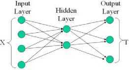
Figure 1. Diagram of a generalized neural network

For the face detection problem, the input vector X will consist of information derived from a color image. The output vector T will be a single number (node) that represents the probability [14] that the image contains a human face. That is, if the pattern to be a human face and observation X a color image, then determine p ( to x ) , or P for simplicity. It should be noted that the interpretation of P as a probability may not hold for actual network output, since there is no guarantee that every input will give rise to an output P such that 0 <  P <  1. the output P for a given input image X as[15]:

> 0.5 ^ X contains a human face

P <  0 . 5   ^ X does not contain a face

, = 0 . 5 ^ unclear if X contains a face

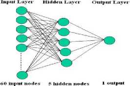
Figure 2. Artificial Neural Network

There are sixty neurons as input, five neurons in hidden layer and one output neuron. The transfer function is sigmoid function [17]. The training data is taken from standard face databases so that it is robust to variations in race, gender and age. The training strategy uses the Levenberg-Marquardt algorithm. LM is more efficient than back-propagation or steepest descent or quasiNewton in to calculating the derivative of the errors in performance with respect to the weight and bias variables.

• III.    Different color spaces and the threshold

VALUE FOR FACE IMAGES

The same training set images of face (20 images) and non-face (18 images) has been used to train the artificial neural network for all the six color spaces which are as RGB, YES, YUV, YCbCr, YIQ and CMY [18]. This training is computed each of the six color spaces YES, YUV, YCbCr, YIQ and CMY for each of the image formats bmp, jpeg, gif, tiff and png. The threshold values for the different color spaces for each image format are obtained from the network outputs graph plotted for each color space. The threshold values are obtained from this graph. The following threshold value table (Table 1) shows the threshold values and the corresponding graphs for each image format.

TABLE I.      T hreshold V alue for different image formats

	RGB	YES	YUV	YCbCr	YIQ	CMY
IF***	bmp	bmp	bmp	bmp	bmp	bmp
TV**	0.8	0.5	0.5	0.5	0.5	0.3
NOP*	Fig3	Fig8	Fig13	Fig18	Fig23	Fig28
IF***	jpeg	jpeg	jpeg	jpeg	jpeg	jpeg
TV**	0.8	0.6	0.6	0.6	0.3	0.4
NOP*	Fig4	Fig9	Fig14	Fig19	Fig24	Fig29
IF***	gif	gif	gif	gif	gif	Gif
TV**	0.5	0.5	0.4	0.5	0.6	0.4
NOP*	Fig5	Fig10	Fig15	Fig20	Fig25	Fig30
IF***	tiff	tiff	tiff	tiff	tiff	Tiff
TV**	0.5	0.4	0.5	0.5	1.5	0.6
NOP*	Fig6	Fig11	Fig16	Fig21	Fig26	Fig31
IF***	png	png	png	png	png	Png
TV**	0.5	0.8	0.5	0.7	0.6	0.5
NOP*	Fig7	Fig12	Fig17	Fig22	Fig31	Fig32

* Network Output plot

** Threshold value

*** Image Format

The histograms were appended to form one input vector X. This paper chose N=20. The Levenberg -Marquardt algorithm was run with the 38 training images of a particular image format for the particular image format concerned determined by various color space histogram approach.

• A.    RGB Color Space Approach for different image formats

The R, G and B are the three colors of the image combined to form any color. The training was performed five times for each of the image formats bmp, jpeg, gif, tiff and png [fig 3-7]. The results for the test data set were encouraging

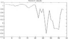
Figure 3. The graph showing output of the neural network for RGB color space for bmp format

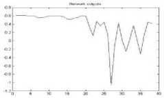
Figure 4. The graph showing output of the neural network for RGB color space for jpeg format

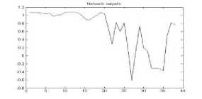
Figure 5. The graph showing output of the neural network for RGB color space for gif format

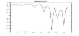
Figure 6. The graph showing output of the neural network for RGB color space for tiff format

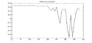
Figure 7. The graph showing output of the neural network for RGB color space for png format

• B.    YES Color Space Approach

The transformation from the standard RGB space to the YES space is given by the equation (1);

Y = 0.253 R + 0.684 G + 0.063 B                                    ^ j ^

E = 0.5 R - 0.5 G

S = 0.25 R + 0.25 G - 0.5 B

In a sense, the Y matrix picks out the edges of the image while the E and S matrices encode the color intensities. The pixel values in the image in three YES relative frequency histograms, each with N equally spaced bins are cataloged. The training was performed five times for each of the image formats bmp, jpeg, gif, tiff and png [fig 8-12]. The results for the test data set were encouraging

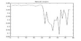
Figure 8. The graph showing output of the neural network for YES color space for bmp format

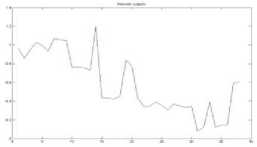
Figure 9. The graph showing output of the neural network for YES color space for jpeg format

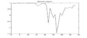
Figure 10. The graph showing output of the neural network for YES color space for gif format

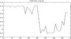
Figure 11. The graph showing output of the neural network for YES color space for tiff format

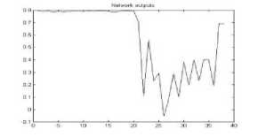
Figure 12. The graph showing output of the neural network for YES color space for png format

• C.    YUV Color Space Approach

A color histogram approach in the YUV color space has been implemented. The transformation from the standard RGB space to the YUV space is given by equation (2).

• D.    YCbCr Color Space Approach

0.299      0.587       0.114 0.615   -0.51499 -0.10001

The color histogram approach in the YCbCr color space is implemented. The transformation from the standard RGB space to the YCbCr space is given by equation (3).

У' и V

-0.14713 -0.28886   0.436

R

G

В

Г = 0.299 хЯ + 0.587х (7 + 0.114x5 + 0СЬ = -0.169 х R - 0.331 х G + 0.499 х В + 128Ст = 0.499 х R - 0.418 х G - 0.0813 х В + 128     (3)

The pixel values in the image in three YUV relative frequency histograms, each with N equally spaced bins are cataloged. The training was performed five times for each of the image formats bmp, jpeg, gif, tiff and png [fig 13-17]. The results for the test data set were encouraging.

The pixel values in the image in three YCbCr relative frequency histograms, each with N equally spaced bins are cataloged. The training was performed five times for each of the image formats bmp, jpeg, gif, tiff and png [fig 18-22]. The results for the test data set were encouraging.

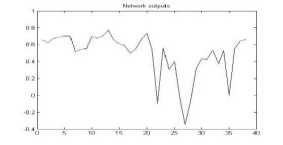
Figure 13. The graph showing output of the neural network for YUV color space for bmp format

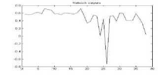
Figure 18. The graph showing output of the neural network for YCbCr color space for bmp format

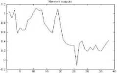
Figure 14. The graph showing output of the neural network for YUV color space for jpeg format

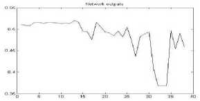
Figure 19. The graph showing output of the neural network for YCbCr color space for jpeg format

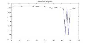
Figure 15. The graph showing output of the neural network for YUV color space for gif format

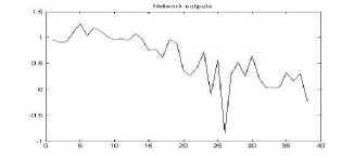
Figure 20. The graph showing output of the neural network for YCbCr color space for gif format

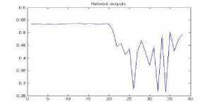
Figure 16. The graph showing output of the neural network for YUV color space for tiff format

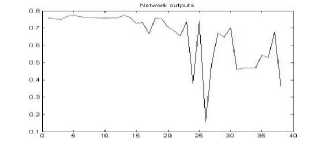
Figure 21. The graph showing output of the neural network for YCbCr color space for tiff format

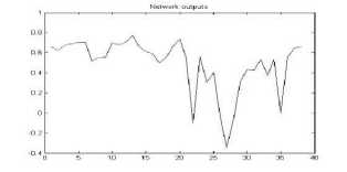
Figure 17. The graph showing output of the neural network for YUV color space for png format

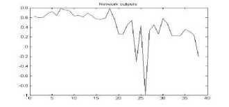
Figure 22. The graph showing output of the neural network for YCbCr color space for png format

• D.    YIQ Color Space Approach

The color histogram approach in the YIQ color space is implemented. The transformation from the standard RGB space to the YIQ space is given by the equation (4).

Y=0.299*R+0.587*G+0.114*B

I=0.596*R-0.275*G-0.321*B

Q=0.212*R-0.523*G-0.311*B              (4)

The pixel values in the image in three YIQ relative frequency histograms, each with N equally spaced bins are cataloged. The training was performed five times for each of the image formats bmp, jpeg, gif, tiff and png [fig 23-27]. The results for the test data set were encouraging

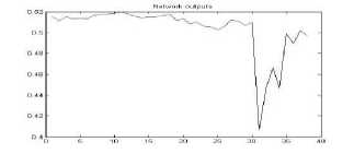
Figure 23. The graph showing output of the neural network for YIQ color space for bmp format

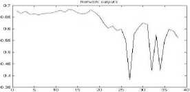
Figure 24. The graph showing output of the neural network for YIQ color space for jpeg format

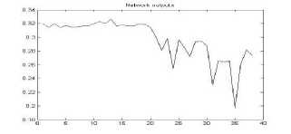
Figure 25. The graph showing output of the neural network for YIQ color space for gif format

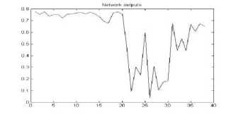
Figure 26. The graph showing output of the neural network for YIQ color space for tiff format

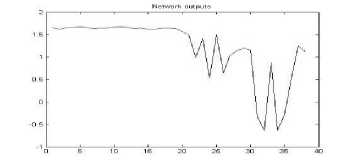
Figure 27. The graph showing output of the neural network for YIQ color space for png format

• E.    CMY Color Space Approach

The color histogram approach in the CMY color space is implemented. The transformation from the standard RGB space to the CMY space is given by the equation (5).

C=1-R

M=1-G

Y=1-B                                   (5)

The pixel values in the image in three CMY relative frequency histograms, each with N equally spaced bins are cataloged. The training was performed five times for each of the image formats bmp, jpeg, gif, tiff and png [fig 28-32]. The results for the test data set were encouraging.

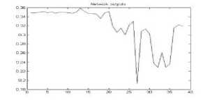
Figure 28. The graph showing output of the neural network for YIQ color space for bmp format

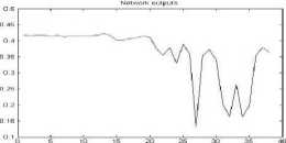
Figure 29. The graph showing output of the neural network for YIQ color space for jpeg format

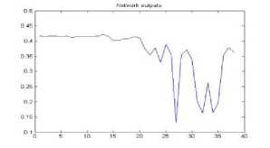
Figure 30. The graph showing output of the neural network for YIQ color space for gif format

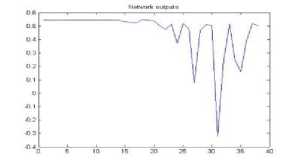
Figure 31. The graph showing output of the neural network for YIQ color space for tiff format

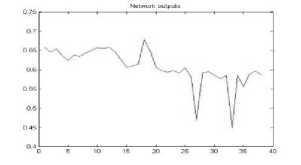
Figure 32. The graph showing output of the neural network for YIQ color space for png format

• IV.  Proposed Algorithm for human face

detection and Location

Step 1: Input image.

Step 2: Repeat steps 3 to 11 until output_value is less than threshold value. The Initial output_value is determined from the output network graph of the concerned color space used

Step 3: Repeat 4 to 11 until window size 100 x 100

Step 4: Select the window size 300 x 300

Step 5: Interpolate the windowed image to 50 x 50

Step 6: Convert RGB values of selected pixels to respective color space and draw Histogram

Step 7: Select 20 intensity levels (bins) to draw the histogram

Step 8: There is 20*3=60 inputs are fed to the artificial neural network, which has three layers, and Levenberg-Marquardt algorithm is used for training.

Step 9: If the value of output from ANN is greater than output_value then it is in facial part and store the co-ordinates of the top left corner of the rectangle and the current window size in database

Step 10: Repeat step 5 to 9 until total image scan is over.

Step 11: Decrease the window size by 50.

Step 12: Decrease output_value by 0.1.

Step 13: If some smaller rectangle gives information same as bigger one then delete smaller rectangle.

Step 14: Display the whole image and draw rectangles using coordinates and windows size from database.

• V.  Experimental results

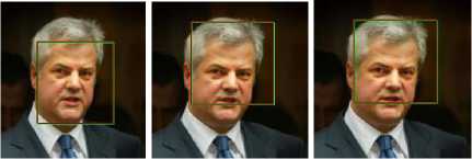
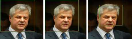
The sample image used for testing is below. The output for different color spaces used for each image format is grouped together as a single figure due to scarcity of space. This image is one of the fifty images chosen for testing. The results for the rest of the images are tabulated later. The results for different image formats are presented according to the order bmp, jpeg, gif, tiff, png. After that the performance for the fifty test images are also calculated. Finally the ratings for the different color spaces are discussed. The face is marked with a red square box. The program after processing the image draws that square over the image while displaying. The original image is left unaltered

Figure 33. Sample Image

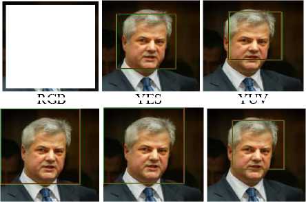
A.1 Output image for Different Color spaces for bmp Image Format

The output image for different color spaces for bmp image format has shown the blow results.

YES

YUV

YCbCr

YIQ

CMY

Figure 34. Output for different color spaces for bmp image format

RGB

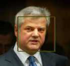
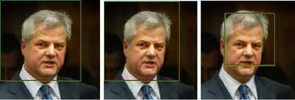
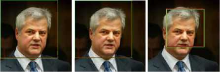
A.2 Output image for Different Color spaces for jpeg Image Format

The output image for different color spaces for jpeg image format has shown the blow results.

RGB       YES        YUV

YCbCr       YIQ         CMY

Figure 35. Output for different color spaces for jpeg image format

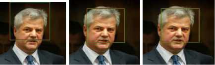
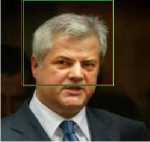
A.3 Output image for Different Color spaces for gif Image Format

The output image for different color spaces for gif image format has shown the blow results.

RGB       YES       YUV

YCbCr      YIQ        CMY

Figure 36. Output for different color spaces for gif image format

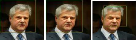
A.4 Output image for Different Color spaces for tiff Image Format

The output image for different color spaces for tiff image format has shown the blow results.

Number of detected face images among test images

Peifoimance =----------------------^-------:-------:—

Niunbei ol test ullages

Accuracy =

Peifoimance

Average Error

The summary for test result of fifty images is as below.

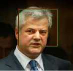
RGB       YES        YUV

YCbCr       YIQ         CMY

Figure 37. Output for different color spaces for tiff image format

A.5 Output image for Different Color spaces for png Image Format

The output image for different color spaces for png image format has shown the blow results.

RGB       YES        YUV

YCbCr        YIQ         CMY

Figure 38. Output for different color spaces for png image format

• B.    Performance of Fifty Test Images Result

The Performance Table (Table II) shows the performance of the six color spaces for 50 test images for each of the image formats bmp, jpeg, gif, tiff, png. The error is calculated by measuring the absolute difference in the size of the window in which the individual program for each color space finds a face and that of the actual size of the face measured in the paint application software. The difference is the error and is shown as a percentage for each color space. The letters D, F and N stands for Detection, No detection and False detection respectively. Based on the average errors for each image format and for each color space, performance and accuracy has been calculated. The two terms performance and accuracy has been described below.

TABLE II.      summary for test result of fifty images

t5	Color Space	No. of faces detected (out of 50 images)			§ м о ^	О > S	о S й Рн	<*
		D	F	N
i	RGB	42	8	0	32.0	0.8	0.84	0.0263
	YES	42	2	6	37.2	0.5	0.84	0.0226
	YUV	46	4	0	23.2	0.5	0.92	0.0397
	YCbCr	32	17	1	53.2	0.5	0.64	0.0120
	YIQ	46	4	0	46.4	0.5	0.92	0.0200
	CMY	45	5	0	47.6	0.3	0.90	0.0190
	RGB	38	12	0	47.2	0.5	0.76	0.0161
	YES	44	6	0	28.0	0.5	0.88	0.0314
	YUV	44	6	0	23.4	0.4	0.88	0.0376
	YCbCr	36	6	8	55.8	0.5	0.72	0.0129
	YIQ	46	4	0	47.8	0.6	0.92	0.0192
	CMY	42	7	1	41.6	0.4	0.84	0.0202
'bf)	RGB	38	12	0	40.6	0.8	0.76	0.0187
	YES	43	7	0	33.0	0.6	0.86	0.0261
	YUV	48	2	0	43.0	0.6	0.96	0.0223
	YCbCr	32	17	1	54.4	0.6	0.64	0.0118
	YIQ	47	3	0	45.6	0.3	0.94	0.0210
	CMY	44	6	0	50.0	0.4	0.88	0.0176
сД	RGB	41	9	0	37.0	0.5	0.82	0.0222
	YES	40	4	6	40.8	0.8	0.80	0.0196
	YUV	46	4	0	25.8	0.5	0.92	0.0356
	YCbCr	30	19	1	56.2	0.7	0.60	0.0107
	YIQ	43	7	0	44.2	0.6	0.86	0.0195
	CMY	44	6	0	43.0	0.5	0.88	0.0205
й5 &	RGB	40	10	0	43.2	0.5	0.80	0.0185
	YES	44	6	0	32.4	0.4	0.88	0.0272
	YUV	46	4	0	22.2	0.5	0.92	0.0414
	YCbCr	34	8	8	59.0	0.5	0.68	0.0115
	YIQ	46	4	0	39.8	1.5	0.92	0.0231
	CMY	41	8	1	43.6	0.6	0.82	0.0188

• C.    Rating of Color Spaces for different image formats

The Tables III and IV shows the ratings of the color spaces based on performance and accuracy. The overall ratings for each of the six color spaces have been computed and the best suitable color space for the purpose of detection and location of human faces in a digital image has been selected. Moreover the ratings of each of the five image formats have been computed and the best suitable image format has been chosen for the same purpose. Based on the tables III and IV tables V and VI have been furnished which shows the Average and Overall ratings of the different color spaces and different image formats. Finally the combination table

(table VII) has been constructed based on tables V and VI. The average and overall ratings and the combination factor are calculated as follows.

• 1.  Average Rating of a color space based on

• 2.  Average Rating of a color space based on

• 3.    Overall Rating of a color space = O r = (P r +A r )/2.

• 4.    Average Rating of an image format based on performance of color spaces =  IFP r =

• 5.    Average Rating of an image format based on accuracy of color spaces = IFA r = (∑Ratings)/6.

• 6.    Overall Rating of an image format = IFO r = (IFP r +IFA r )/2.

• 7.    Combination Factor = C f = (O r +IFO r ).

performance = P r = (∑Ratings)/5.

accuracy = A r = (∑Ratings)/5.

(∑Ratings)/6.

TABLE III.    Ratings of the six color spaces based on performance for the Different Image Formats

VD	Ratings
	6	5	4	3	2	1
Ph 8	YUV YIQ	CMY	RGB YES	YCb Cr
ад .Ph	YIQ	YUV YES	CMY	RGB	YCb Cr
"Й	YUV	YIQ	CMY	YES	RG B	YC bCr
	YUV	CMY	YIQ	RGB	YES	YC bCr
Ph	YUV YIQ	YES	CMY	RGB	YCb Cr

TABLE IV.    Ratings of the six color spaces based on accuracy for the Different Image Formats

Image Format	Ratings
	6	5	4	3	2	1
bmp	YUV	RGB	YES	YIQ	CMY	YCb Cr
jpeg	YUV	YES	CMY	YIQ	RGB	YCb Cr
gif	YES	YUV	YIQ	RGB	CMY	YCb Cr
tiff	YUV	RGB	CMY	YES	YIQ	YCb Cr
png	YUV	YES	YIQ	CMY	RGB	YCb Cr

TABLE V.     Average and Overall Ratings of the six color spaces based on performance and accuracy for the Different Image Formats

	YUV	YIQ	YES	CMY	RGB	YCbCr
P r	5.8	5.4	4.4	3.8	3.0	1.8
A r	5.8	3.2	4.6	3.0	3.4	1.0
O r	5.8	4.3	4.2	3.7	3.2	1.4

TABLE VI.    Average and Overall Ratings of the five image formats based on performance and accuracy for the Different Color Spaces

	bmp	png	jpeg	tiff	gif
IFP r	4.67	4.33	4.17	3.50	3.50
IFA r	3.50	3.50	3.50	3.50	3.50
IFO r	4.085	3.915	3.835	3.500	3.500

TABLE VII. C ombination T able

	YUV	YIQ	YES	CMY	RGB	YCbCr
bmp	9.885	8.385	8.285	7.785	7.285	5.485
png	9.715	8.215	8.115	7.615	7.115	5.315
jpeg	9.635	8.135	8.035	7.535	7.035	5.235
tiff	9.300	7.800	7.700	7.200	6.700	4.900
gif	9.300	7.800	7.700	7.200	6.700	4.900

• VI. Conclusion and Future Work

The YUV color space has been more accurately detected the faces in the images for the bmp image format. The result of the combination of the color space with that of the image format is clear from the Combination Table (Table VII). For further works, the combination of the YUV color space and bmp image format should be studied more vividly. The present work may be extended with the location of images and its performance for faces inclined at some angle within an image. However the mixing of the image formats for training images may show some unexpected results which may be positive or negative. Moreover training the neural network for more number of bmp images for the YUV color space should be studied. Some inherent obstructions in this method are that using an interpolated image resulting in loss of information, proper selection of intensity levels (which in this case is 20) and also this method is concerned with the average distribution of colors. So the algorithm will lead to skin detection rather only face detection. The following input output implies that there are three faces and one false detection [Fig 39]. The reason is simple the rectangle of the false detection contains within itself a major portion of skin color and hence the average value of the histogram lies within that of the values for face and hence the output.

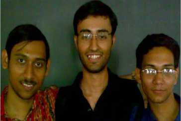
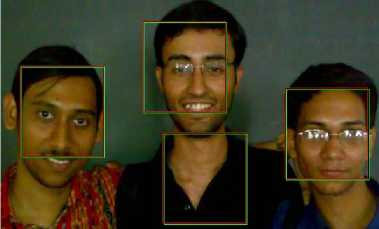
Figure 39. Input and Output Images (False Detection)

• [9]    Y. Dai and Y. Nakano. Face-texture model based on SGLD and its applications in face detection in a color scene. Pattern Recognition , 29 (6) (1996), pp. 1007-1017.

• [10]    Q. Chen, H. Wu, and M. Yachida. Face detection by fuzzy pattern matching. Proceedings of the Fifth International Conference on Computer Vision , 1995, pp. 591-596.

• [11]    J. Cai and A. Goshtasby. Detecting human faces in color images. Image and Vision Computing , 18 (1999), pp. 63-75.

• [12]    Y. Miyake, H. Saitoh, H. Yaguchi, and N. Tsukada. Facial pattern detection and color correction from television picture and newspaper printing. Journal of Imaging Technology , 16 (5) (1990), pp. 165-169.

• [13]    D. Androutsos, K.N. Plataniotois, and A.N. Venetsanopoulos. A novel vector-based approach to color image retrieval using a vector angular-based distance measure. Computer Vision and Image Understanding , 75 (1/2) (July/August 1999), pp. 4658.