Performance Analysis of Alpha Beta Filter, Kalman Filter and Meanshift for Object Tracking in Video Sequences

Published Online February 2015 in MECS

Object tracking is an important task within the field of computer vision [1]. From video surveillance to image processing, object tracking finds its applications in many areas. Object tracking which was once largely used for military and defense purposes is now rapidly finding its feet in commercial and industrial sector. For example, different sports like tennis and cricket have adopted the ball tracking technique (Hawk eye) in order to promote accurate decisions. Also, many CCTV cameras equipped with object tracking algorithms are being deployed on the roads in order to maintain and regulate traffic flow [1]. Another important area of application for object tracking is video surveillance where extraction of motion information is not only possible but also detection of any suspicious activities or unlikely events [1]. However, tracking of objects is very complex in nature due to several problems such as presence of different noise in video, motion of objects, non-rigid or articulated nature of objects, partial and full object occlusion, changes in scene illumination and background [1].

To address these problems many performance metrics have been developed which take into account different parameters and conditions. Thus, evaluating the performance of tracking algorithms is becoming increasingly important and is an on-going research topic especially in video sequences. In this paper, we have focused our research in evaluating the above mentioned algorithms against their Root mean square error RMSE, Object tracking error OTE, Tracking detection rate, Peak signal to noise ratio PSNR, Boundary box error, error plots and time taken per frame in normal and noisy conditions. The algorithms have been simulated in MATLAB and results are analyzed and summarized.

The paper has been structured as follows: Section II gives the overview of the object tracking system, Section III presents the state modelling of the object, Section IV describes the different algorithms used, Section V discusses the evaluation measures and compares the object tracking methods and Section VI presents the concluding remarks of the paper.

• II.    Object Tracking System In Video Sequences

Tracking a moving object from a given video is done by extracting a sequence of images from the video at a given frame rate. After acquiring the sequence of images, detection of the object in every frame is done by distinguishing the foreground image from the background image using an object detection technique. Once the segmentation of the regions and detection of the object is achieved, we then employ tracking algorithms to track the objects from one frame to the next and generate its trajectory over time. An overview of this system described above is shown in Fig 1 [2]. After noting the tracked object’s parameters, we proceed with evaluating each algorithm performance.

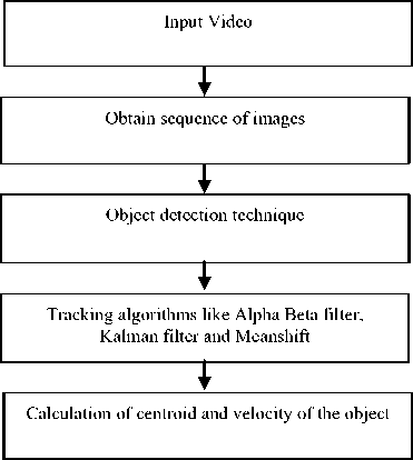
Fig 1. Object tracking system

• III.    Mathematical Modeling

Before we proceed with tracking an object, it is mandatory to model our system. This is done using the process state space equation given by (1). In this paper, we have modeled our system using the constant velocity model.

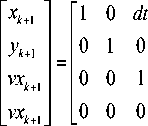
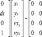
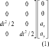
Where x k+1 and y k+1 are the x and y coordinates of center of object at the instant, x k and y k are the x and y coordinates of center of object at previous instant, vx k+1 and vy k+1 are the x and y component of velocity at the instant, vx_k and vy_k are the component of velocity at previous instant and a_x and a _y are accelerations of the object in x and y direction.

Since we have used the constant velocity model, the acceleration terms can be taken as process noise wk. Thus, the above equation (1) can be written as (2), xk+1 = Axk+ wk

Where A is called the state transition matrix and w k is the Process noise given by w k ~ (0, Q) which is assumed as zero mean white Gaussian noise with process noise covariance Q.

Next step is to model the measurement space which is given by the measurement equation given below, xk+1

. Ук + 1

xk + vk * randn yk vk * randn

which can be written as (4)

z k = Hx k + v k              (4)

Where z k is called the measurement vector, H is known as the measurement transition matrix and v k is called the measurement noise given by v k ~ (0, R k ) which is assumed as zero mean white Gaussian noise with measurement noise covariance R k .

• IV.    Object Tracking Algorithms

• A.    Alpha Beta filter

Alpha Beta tracker is similar to Kalman filter but a simplified form of it. Unlike the Kalman filter it uses a simple static system model. It is generally used for steady state stationary condition in which tracking is characterized by constant velocity of the object and constant measurement noise covariance.

It is implemented using two steps - i) Prediction and ii) Correction. The former step includes the prediction of the current set of object parameters that is the position and velocity estimate. An error is calculated based on the true and predicted values of object parameters. The error in position and velocity predicted is corrected using the static Alpha and Beta gains respectively. Alpha and beta gains are initialized in the beginning of the algorithm.

The underlying alpha beta model described above is represented by mathematical equations from (5) to (8) [3][4][5].

Prediction:

xk = xk-i+ Tvk-i vk = vk-i

Correction:

xk = xk + a(xk - xk—)

Vk = Vk + (в / T)(Xk - Xk—)(8)

Where x k is the predicted position, x k-1 is the previous position; v k is the predicted velocity of object and v k-1 is the previous velocity of object; x k^- is the true position of the object, x k -x k^- is the amount of error in prediction, α and β are called the Alpha and Beta gains respectively and T is the sampling period.

• B.    Kalman filter

Kalman filter is a recursive filter that provides efficient tracking estimations of the object even in presence of Gaussian noises [6]. It uses a detailed dynamic system model compared to that of Alpha Beta filter. Kalman filter because of its small computation requirement and efficient recursive property is popularly used as an optimum tracking algorithm in various fields [6]. The algorithm is implemented using two steps – i) Prediction ii) Correction.

Initially, state transition matrix A , Process noise covariance Q , measurement noise covariance R and measurement transition matrix H are initialized. The next step involves the prediction of the present state of the object and error covariance described by equations from (9) to (11) [6][7][8][9]. This predicted state estimate is called the priori estimate. The state of the object is represented by 4x1 state matrix x given by [x y v x v y ] where x and y represent the coordinates of the object and v x and v y represent the object’s velocity in x and y direction respectively.

Prediction:

xk - = Axk-1 + wk-1

Pk - = APk—1 A + Q(10)

p(w)  N (0,Q)

Where, A is called the state transition matrix, x k-1 is the previous state, x k^- is the predicted state, P k^- is the predicted error covariance, P k-1 is the previous error covariance and Q is called the process noise covariance.

Next, the Kalman filter uses the state prediction x k^- and error covariance at k instant to correct its prediction by using Kalman gain K . This corrected estimate is called posteriori estimate which is described by equations from (12) to (15) [6][7][8][9]. The equations in-cooperate a new measurement into the priori estimate to obtain an improved posteriori estimate. z k is the true state of the object’s x and y coordinates and H is the measurement transition matrix which maps the observed space from true space.

Correction:

K = P - HT (HPk - HT + R ) 1(12)

xk = xk"+ K(zk - Hxk " )

Pk = (I - KH)Pk- p(v)  N(0,R)(15)

Where K is the Kalman gain, P k^- is the predicted error covariance, H is the measurement transition matrix, R is the measurement noise covariance, x k is the corrected state, z k is the measurement matrix and P k is the corrected error covariance.

From the above equations it is evident that the Kalman filter takes into the dynamics of the environment by considering the noise covariance.

C. Meanshift algorithm

Mean shift is a nonparametric iterative algorithm [10][11]. It iteratively shifts the data point to the average of data points in its neighborhood. For each data point, mean shift defines a window around it and computes the mean of data point. Then it shifts the center of window to the mean and repeats the algorithm till it converges [10].

Given n data points x i , i= 1,2……n on a d dimensional space R ^d ,the multivariate kernel density estimate obtained with Kernel K(x) and window radius h is given by (16).

f (x) = A £k I x xi nh X ( h

The radially symmetric kernel is defined by (17)

K ( x ) = C k k (|| x ||²)               (17)

Where c k is the normalization constant. Taking the gradient of the density estimator and further algebraic manipulation yields,

2 c

V f ⁽ x >  = nh^

n

X g i=1

i h

*

JL^    I

^X xg I

n

X g i =1

Where g(x) = -k ^’ (x) denotes the derivative of the selected kernel profile. The first term is proportional to the density estimate at x (kernel G = c_gg (|| x ||² ) ). The second term is the mean shift vector M which points to the direction of maximum increase in density. The mean shift algorithm is summarized as follows:

• i)    Compute mean shift vector M ( x^t ).

• ii)  Translate  density estimation window  using

x t ^{+ 1} = x t + M ( x t )

• iii)    Iterate the above steps i) and ii) until they

convergence i.e. V f ( x ) = 0

• V. Experiemental Simulation And Results

• A.    Video Specifications

Video length: 2.4 sec

Image dimension: 1270*720 pixels

Image type: RGB color space

Height: 720 pixels

Width: 1280 pixels

No of frames: 73

No of frames with object: 36

• B.    Experimental Results

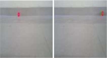
Fig 2. Alpha Beta tracking under normal conditions

Fig 6: Kalman tracking under noisy conditions

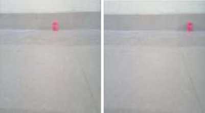
Fig 7: Meanshift tracking under noisy conditions

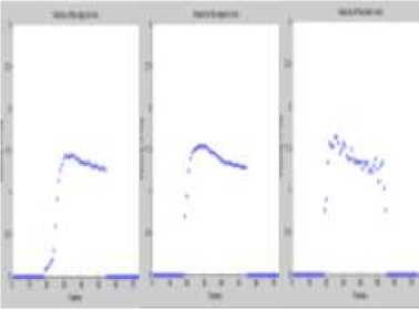
The position estimate is plotted in Fig 8 under normal conditions. Red indicates the object tracked and Blue indicates the actual position of the object.

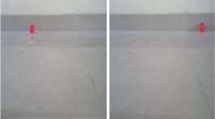
Fig 3. Kalman tracking under normal conditions

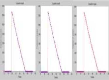
(a)                       (b)                       (c)

Fig 8. (a) αβ filter ( b) Kalman filter (c) Meanshift position estimate

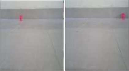
Fig 4. Meanshift tracking under normal conditions

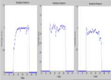
The velocity estimate for the tracking algorithms is plotted in Fig 9 under normal conditions. The true average velocity of the object is 1.375m/s. The estimated average velocity for αβ filter is 1.117m/s, Kalman filter is 1.371m/s and Meanshift is 1.362m/s.

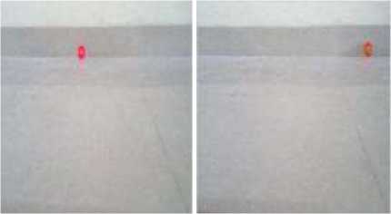
Fig 5: Alpha Beta tracking under noisy conditions

(a)                       (b)                       (c)

Fig 9. (a) αβ filter (b) Kalman filter (c) Meanshift velocity estimate.

Now that we know the true and tracked object’s parameters, we can evaluate their performance. In this paper we have compared the tracking algorithms using the following set parameters. Although there are many metrics in evaluating the tracking performance, we have limited to the following seven parameters as they can implemented with ease.

B.A. Absolute error

Absolute error is the magnitude of difference between the true value and the tracked value of the object. It is given by,

^ I o true    o tracked

Where o true is the true value of object’s parameters and o tracked is the tracked value of the object’s parameters.

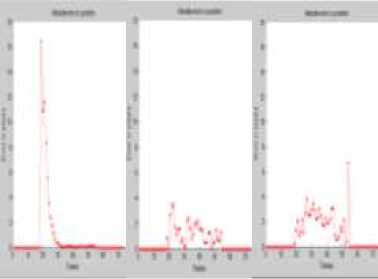
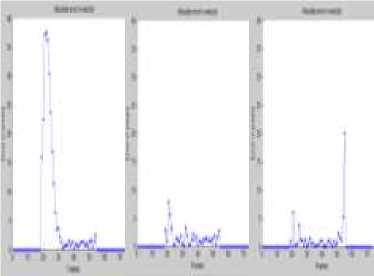
The absolute error in position and velocity is shown in Fig 11 and Fig 12 respectively for the three tracking algorithms. We can notice that Kalman filter has the least error in estimating the object’s position and velocity.

B.B. Root Mean Square Error

RMSE measures the difference between values predicted and the values actually observed. It is given by,

RMSE =

n

^^ ⁽ o pr'edc'ted    o observed )

i =1

n

Where o predicted is the tracked estimation of the object’s parameters, o observed is the true estimation of the object and n is the number of frames with the object present.

The RMSE in position and velocity is tabulated in Table I and II under normal and noisy conditions. We can notice that Kalman filter has the lowest RMSE error, followed by Mean shift and Alpha Beta filter which has the highest RMSE error in normal and noisy conditions.

B.C. OTE error

Object tracking error (OTE) is the average discrepancy in the centroid of the tracked object from its true value. It is given by [12],

OTE =

xtracked )   + ⁽ yruee

—

y tracked )

n

Where x true and y true are the actual x and y coordinate of the object, x tracked and y tracked are the tracked x and y coordinate of the object.

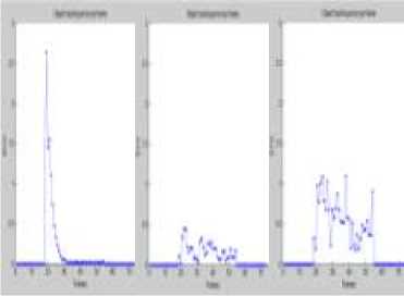
Since the errors in determining position is least for Kalman followed by Mean shift and Alpha Beta filter. The OTE for Kalman is expected to be least among the other two tracking algorithms in noisy and normal conditions. The values are summarized in Table I and II and OTE per frame is plotted in Fig 13.

B.D. Tracking detection rate

Tracking detection rate refers to the amount of success in detecting an object [14].

TDR =

no of frames object detected no of frames with object present

*100

From the Table I and II, it is evident that all the three algorithms have good tracking rate in normal conditions as opposed to noisy conditions where there are missed detections.

B.E. Bounding box error

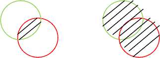
Bounding box error refers to the overlap area error of the tracked object to the actual object [13]. If BBE is 1, then the tracking is accurate to the true object location and size and 0 indicates the worst performance of the tracking algorithm i.e. no object tracked.

BB_E = Area ( A и T ) Area ( A n T )

Where A i s the true area of the object and T is the area of the object tracked. Fig 10 shows an object outlined by green and object tracked outlined by red. The shaded areas represent intersection and union of A and T respectively.

(a)                           (b)

Fig 10. (a) A ∩ T (b) A U T

From the Fig 14, we notice that Kalman Filter performs better in detecting the object and has less BBE as compared to the other algorithms.

To evaluate the performance in noisy conditions, we use Peak signal to noise ratio which gives ratio between the maximum possible power of a signal and the power of corrupting noise.

Alpha Beta requires a high PSNR of about 19 db for tracking the object in noisy conditions reasonable well whereas Kalman and Mean shift both perform even better at that value. The min PSNR required for Mean shift is 16 db and for Kalman is 15 db. Thus, we conclude that Kalman filter performs well in low values of PSNR. The performance for a given PSNR value is summarized in Table II.

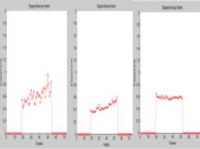
By evaluating the time taken to track the object we can determine which algorithm can work faster. Fig 15 shows the time taken to track the object per frame. We notice that Kalman takes overall less time per frame to track the object location compared to Meanshift and Alpha Beta filter.

(a)                       (b)                       (c)

(a)                       (b)                       (c)

Fig 15. (a) αβ filter (b) Kalman filter (c) Meanshift Time taken per frame.

Fig 11. (a) αβ filter (b) Kalman filter (c) Meanshift Absolute error in position per frame.

(a)                       (b)                       (c)

Fig 12. (a) αβ filter (b) Kalman filter (c) Meanshift Absolute error in velocity per frame.

(a)                       (b)                       (c)

Fig 13. (a) αβ filter (b) Kalman filter (c) Meanshift OTE per frame.

(a)                       (b)                       (c)

Fig 14. (a) αβ filter (b) Kalman filter (c) Meanshift Bounding Box error.

TABLE 1. Under Normal Conditions

Algorithm	Performance parameters
	RMSE Position (cm)	RMSE Velocity (cm/s)	OTE (cm)	TDR
αβ Filter	0.5473	1.7803	0.7532	35/36= 97.22%
Kalman filter	0.2002	0.2867	0.1642	36/36= 100%
Meanshift	0.3012	0.4764	0.6748	36/36= 100%

Table 2. Under Noisy Conditions

Algorithm	Performance parameters
	RMSE Position (cm)	RMSE Velocity (cm/s)	OTE (cm)	TDR	PSNR (db)
αβ Filter	23.971	26.971	33.346	33/36= 91.66%	18.39
Kalman filter	0.3012	0.4013	0.1721	36/36= 100%	18.39
Meanshift	0.5059	0.6351	1.0380	36/36= 100%	18.39
αβ Filter	0.5729	1.9203	1.7969	35/36= 97.22%	20.15
Kalman filter	0.2012	0.2967	0.1670	36/36= 100%	20.15
Meanshift	0.4920	0.6348	0.7449	36/36= 100%	20.15

• VI. Conclusions

Comparing and evaluating the simulation results for Alpha beta filter, Kalman and Meanshift the following conclusions can be drawn regarding their performances. Firstly, Kalman filter has the least error in calculation of the object trajectory compared to Meanshift and Alpha beta filter. Thus, as expected the OTE and RMSE errors for Kalman are quite low. Secondly, Kalman filter can precisely detect and track the ball and hence provides the least boundary box error compared to the other algorithms. Lastly, Alpha Beta performs the worst in noisy conditions and needs a high value of PSNR to work reasonably well. Overall, Kalman filter is preferable over Meanshift and Alpha beta filter.