Performance Analysis of Cluster-based Wireless Sensor Networks with Application Constraints

Published Online October 2009 in MECS

Advances in wireless communications and electronics have fostered the development of relatively in-expensive and low-power wireless sensor nodes that are extremely small in size and communicate un-tethered in short distances. Wireless sensor node is a battery-operated device, capable of sensing physical quantities, data storage, limited amount of computational and signal processing capability and wireless communication. A Wireless Sensor Network (WSN) is composed of a large number of sensor nodes that are densely deployed either inside the phenomenon or very close to it [1]. WSN can have one or more sinks or Base Stations (BS) which collect data from sensor nodes. These sinks act as an interface through which the WSN interacts with the outside world. WSNs facilitate monitoring and controlling of physical environments from remote locations with better accuracy. Sensor nodes in WSNs have various energy and computational constraints because of their inexpensive nature and ad-hoc method of deployment. They usually employ performance metrics that are different from those of conventional networks, emphasizing on low power consumption and low cost rather than data throughput or channel efficiency. Major advantages of WSNs over the conventional networks deployed for the same purpose are greater coverage, accuracy, reliability and all of the above at a possibly

Manuscript received January 18, 2009; revised June 13, 2009; accepted July 22, 2009.

lower cost. Some of the early works on WSNs have discussed these benefits in detail [2], [3], [4].

WSNs have innumerable number of applications in various fields triggering a great deal of research attention in recent times. Several applications have already been envisioned for these types of networks ranging form environment, agriculture, industry, object detection, its classification and tracking, disaster relief, facility management, preventive maintenance, medicine and health to name the few [5], [6], [7], [8]. WSN applications can be classified according to the nature of the functionalities, and in addition according to the data delivery and communication pattern between the sensor nodes and the base station [9]. According to their functionalities, WSN applications can be classified into four main categories: monitoring applications, tracking applications, controlling applications, and hybrid applications.

Based on the data delivery and communication pattern between the sensors nodes and the base station (sink), WSN applications can be classified into four classes: The continuous model on which sensor nodes periodically report to the observer about a physical parameter. For example, nodes in a network monitoring precision agriculture are periodically sending temperature, light levels, and soil moisture to the observer over a multi-hop network. The event-driven model where sensors send information only if an event of interest is detected. For example, sensors that are deployed to detect forest fires will report only when the temperature exceeds a certain degree. The observer-initiated model on which the observer may be interested only in the occurrence of an event at certain geographic area. In this case, the observer will send an explicit request to specific sensors. Note that such query can be predefined in advance by the application to be answered by specific sensors at certain intervals. This can be viewed as a prescheduled observer-initiated model. The hybrid model where some or all of the above three models coexist in the same network.

Although formation and maintenance of clusters introduces additional cost due to the control messages required for the purpose, still cluster-based WSNs have taken much attention of the researchers due to their better performance. Distributed, dynamic and randomized clustering schemes are interesting due to their simplicity, feasibility, and effectiveness in providing energy-efficient utilization, load balancing and scalability simultaneously [10]. Being a dominant representative in this class, LEACH (Low Energy Adaptive Clustering Hierarchy) [11], [12] has attracted intensive attention and become a well studied and popularly referred baseline since its appearance. Much work [13], [14], [15], [16] has been carried out to enhance LEACH.

In order to evaluate the performance of the LEACH protocol, the authors used a communication model where nodes always have data to send to the end user and nodes located close to each other have correlated data. In other words the authors used an event-driven model where the event was occurring always and every where all around the sensor field. Simulation results presented in [11] do indicate the better performance of the LEACH protocol over static clustering and MTE (Minimum Transmission Energy) protocol [17], [18] for such communication patterns. In order to further optimize the performance of the LEACH protocol, their remains a need to evaluate the performance of the LEACH protocol for different communication patterns formed due to the application constraints for WSNs.

In this paper we have carried out the performance analysis of cluster-based WSNs based upon LEACH protocol for different communication patterns between the sensor nodes and the base station due to application constraints. The main focus is to identify the factors that affect the network lifetime by inducing unbalanced energy consumption among sensor nodes for different communication patterns due to application constraints. The remainder of the paper is arranged as follows. Section-II provides the background about cluster-based WSNs based upon LEACH protocol. The details of the proposed scenarios based upon the different communication patterns formed due to application constraints that were chosen for the performance evaluation by developing a simulation environment has been discussed in section-III. Methodology for the development of the simulation environment using OPNET to identify the factors inducing unbalanced energy consumption among sensor nodes and thus affecting the network lifetime has been discussed in section-IV. Based upon the simulation results, conclusions have been drawn and some recommendations for future work have been proposed in section-V.

• II.    Brief Review of LEACH

LEACH [11], [12] is a distributed clustering protocol that utilizes randomized rotation of local CHs to evenly distribute energy consumption among sensor nodes in the network. In LEACH, the whole operation is divided into many rounds. Every round includes a set-up phase followed by a steady-state phase. During the set-up phase, nodes are organized into clusters with each cluster having its own CH through short message communications using Carrier Sense Multiple Access (CSMA) MAC protocol. Each CH sets up TDMA schedules for its member nodes which are later used to exchange data between the member nodes and the CH during steady-state phase. The steady state phase consists of many frames. Since the duration of each slot in which a node transmits data is constant, so the time to send a frame of data depends on the number of nodes in the cluster. Data are transferred from member nodes to CHs according to the assigned TDMA schedules during each frame, aggregated to reduce redundant data and then passed on to the BS. Fig. 1 shows the round timeline diagram for the LEACH protocol. To reduce inter-cluster interference, members of each cluster communicate using Direct-Sequence Spread Spectrum (DSSS).

LEACH forms clusters by using a distributed algorithm, where nodes make autonomous decisions without any centralized control. Each node elects itself to be a CH at the beginning of round r with probability P_i(t) such that the expected number of CHs for that round is k . Thus, if there are N nodes in the network

N

E ( CH ) = £ P ( t )*1 = k (1) i = 1

To ensure that all nodes are CHs the same number of time, LEACH protocol requires each node to be a CH once in N/k rounds on average. If Ci(t) is the indicator function determining whether or not node has been a CH in the most recent ( r mod N/k ) rounds (i.e. Ci(t)=0 if node has been a CH and one otherwise), then each node should choose to become a CH at round r with probability

k

C ( t ) = 1

Pt (t ) = ^

N - k *( r mod N / k )

C ( t ) = 0

• A. Rad o Energy D ss pat on Model

For simplicity LEACH proposes a simple model for the radio hardware energy dissipation where the transmitter dissipates energy to run the radio electronics and the power amplifier, and the receiver dissipates energy to run the radio electronics, as shown in Fig. 2. For the analytical and simulation work described in this paper, both the free space (d2 power loss) and the multipath fading (d4 power loss) channel models were used, depending on the distance between the transmitter

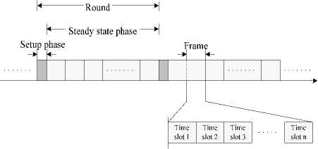
Figure 1: Round timeline diagram for LEACH protocol

TABLE I. R adio M odel C ommunication P arameters

Parameter name	Value
RF Radio circuitry energy ( E elect )	50 nJ/bit
Amplifier energy for Free space loss ( ε fs )	10 pJ/bit/m2
Amplifier energy for Multipath loss ( εmp )	0.0013pJ/bit/m4
Threshold distance ( d0 )	87m
Data aggregation energy ( EDA )	5nJ/bit/signal

III. Details of the Proposed Scenarios

and receiver. Power control can be used to invert this loss by appropriately setting the power amplifier. If the distance is less than a threshold, the free space model is used; otherwise, the multipath model is used. Thus, to transmit an l-bit message a distance d , the radio expends

E Tx ( ^l , d ) = E Tx _ elect ( ^l ) + E Tx amP ( ^l , d )

lE elect + l ^£ fs d 2

lE elect + ^{l e}mp d 4

d <  d 0

d >  d 0

and to receive this message, the radio expends

E rx ( l) = E rx _ elect ( l ) = ^lE elect

The lifetime of a WSN can be defined as the time elapsed until the first node dies, the last node dies, or a fraction of nodes die [4], [19]. In a WSN, in addition to minimizing energy expenditure, a protocol design should also take fairness into consideration to achieve a sharp edge effect [19], i.e. individual nodes drain out of energy at similar time. Thus when the network loses its functionality, remaining active nodes should have little residual energy. An ideal scheme should enable the network to operate for the longest possible time, while each node burns its energy at the same pace. Our objective is to determine how much extent LEACH

Table 1 summarizes different communication energy parameters as proposed in [11] used in the simulation work described in this paper.

B. Traffic Patterns of the LEACH Protocol

As previously mentioned, in order to evaluate the performance of the LEACH protocol, the authors used a communication model where nodes always have data to send to the end user and nodes located close to each other have correlated data. In other words the authors used an event-driven model where the event was occurring always and every where all around the sensor field. So in order to make effective use of bandwidth resources CHs in any round divide the round time into frames where frame duration and hence the number of frames per round for each cluster depends upon the number of member nodes in that cluster, i.e. Small clusters will have more frames per round and vice versa. Such traffic patterns cover only a limited number of scenarios for WSN applications. Considering the classification of WSN applications based upon the data delivery & communication pattern between the sensor nodes and the base-station, there can be wide range of scenarios following the continuous model, event driven model, observer initiated model and hybrid model.

protocol achieves sharp edge effect and what are those factors that induce unbalanced energy consumption among sensor nodes and hence affect the network lifetime.

For the simulation work described in this paper, we used a 100-node network with the same network specifications as were used in [11]. The bandwidth of the channel was set to 1 Mb/s, each data message was 500 bytes long, and the packet header for each type of packet was 25 bytes long. Table II summarizes different network parameters.

From energy consumption perspective, as per LEACH specifications, each CH node dissipates energy receiving signals from its member nodes, aggregating the signals and transmitting the aggregated signal to the BS. Assuming that the BS is far from the sensing area, the energy dissipation follows the multipath model ( d⁴ power loss). So the energy dissipated by the CH ( E CH ) during a single frame is

E CH = ^{l E}elect f ^ “1^ + ^lEDA ^ ^{+ lE}elect ^{+ l £} mp^dtoBS ⁽⁵⁾

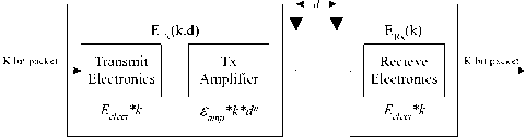
Figure 2: Radio energy dissipation model

(N/k-1) is the average number of non-CH nodes in each cluster with k clusters in each round.

Each non-CH or member node only needs to transmit its data to the CH once during each frame. Presumably the distance to the CH is small, so the energy dissipation follows the free-space model ( d² power loss). Thus, the energy dissipated in each non-CH node ( E non-CH ) during a frame is

E non - CH

= ^lE elect ^{+ l £} fs

1 M ²

2 n k

M²/2πk is the average squared distance of the non-CH nodes from their CH.

TABLE II. S ensor N etwork P arameters

Parameter	Value
Sensing area (M)	100 X 100
Number of sensor nodes (N)	100
D toBS (min)	75
D toBS (max)	185
Initial node energy level (E init )	2.0 J
Data packet size ( l )	4000 bits

For the simulation work described in this paper, we used event driven communication model and continuous communication model. Following are the details of these communication models.

• A.    Event Driven Model

In order to evaluate the performance of the LEACH protocol, the authors used a communication model where nodes always have data to send to the end user and nodes located close to each other have correlated data. This corresponds to an event-driven model where the event was occurring always and every where all around the Sensor Field (SF). In general there can be scenarios where the Event Field (EF) is confined within a certain region in the SF. For example sensor nodes are deployed to detect the forest fire but the fire is confined within a certain region of the overall SF. Fig. 3 describes those kinds of scenarios.

For all those scenarios in which the EF is confined within a certain region of the SF, only those member nodes which are located inside the EF have data to send to their CHs. In general this gives rise to three possible scenarios.

Cluster fully confined within the Event Field: In this case, since all the members of a cluster are located inside the EF so all the non-CH nodes will detect that event and then transmit this information to the BS and dissipate energy for this transmission activity. CH nodes will dissipate energy while receiving signals from member nodes, aggregating those signals and then communicating the aggregated data to the BS as given in equation 4 during each frame.

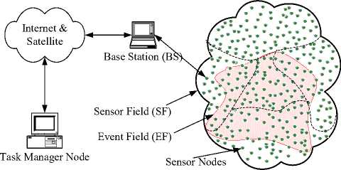
Figure 3: A WSN scenario where the event field is confined within a certain region of the sensor field

Cluster located outside the Event Field: In this case, all the members of a cluster are located outside the EF.

Since all the non-CH nodes will not detect any event so they will not have any information to transmit to the CH and hence all these nodes will not dissipate any energy in this aspect. On the other hand the CH node has to keep its receiver on for any possible communication from its member nodes so it will be consuming reception part of the energy. During its own time slot for data transmission to the BS, since is does not have any data to aggregate and report to the BS so it will not be consuming any energy due to data aggregation and BS transmission.

Cluster partially confined within the Event Field: In this case, some of members of the cluster are located inside the EF while the others are located outside the EF.

Only those non-CH nodes which are located inside the EF will detect that event and then transmit this information to their CH and dissipate energy for this transmission activity. Those non-CH nodes which are located outside the EF, will not detect any event so they will not have any information to transmit to their CH and hence these nodes will not dissipate energy in this regard. The CH node has to keep its receiver on for any possible communication whether it is there or not so the reception part of the energy will be there. During its own time slot for data transmission to the BS, it has to aggregate the only that information which it received from those member nodes which were located inside the EF along with its own information if it is also located inside the EF and has to transmit the aggregated information to the BS.

We define E/S as the ratio of the EF area to the SF area.

For example E/S = 0.2 means EF is confined only to the 20% of the total SF. For the sake of simplicity if we assume that the EF is confined in the form of a circle from the centre of the SF and if A is the total area of the

SF, then for a particular value of the E/S, we can calculate the radius of the EF (R EF ) as follows

R EF =

E

A X —

S

П

Using different values of E/S, we can determine the corresponding radius of the EF. Nodes located within the circle will be able to detect the event and report the sensed value to their CH.

• B.    Continous Model

For a broader range of WSN applications sensor nodes can be tasked with periodic reporting of the measured values. The reporting period for the measured values is an application dependent parameter. Number of frames per round will not vary with the cluster size as was the case with an event driven model. Under the ideal circumstances, the number of frames value should be set such that each node should act as CH only once during the network lifetime. In order to have a detailed analysis of the LEACH protocol for the continuous model, we set three different values of number of frames per round such that each node should have CH role assignment once, two times and four times respectively.

• IV.    Simulation Work

Based upon the specifications of the LEACH protocol from section II and objectives for the proposed work defined in section III, there is a need to carry out the performance analysis of the LEACH protocol for different communication patterns formed due to application constraints. OPNET was chosen as the simulation platform. This tool is a discrete-event simulator developed by MIL3 Corporation and it provides a comprehensive development environment for the specification, simulation and performance analysis of communication networks. As a building block, a sensor node model was developed. The base scenario of the simulation environment comprised of 100 randomly distributed nodes in a sensing area of 100×100 m2 and a BS located outside the sensing area as per network specifications listed in table II.

Fig. 4 (a) and (b) show the total number of effective data signals received at the BS over time and total effective data received at the BS for a given amount of energy respectively for different values of E/S. For smaller values of E/S, only nodes present inside the EF reported the information to their corresponding CH which transferred this information to the BS. For all those clusters in which all the members are located outside the EF , even though the non-CH are not dissipating any energy for transmission as they don’t detect any event but still their corresponding CH has to dissipate energy as it has to keep its receiver on for the possible communication from its member nodes, but at the end of the frame as the CH node don’t have any data to transmit to the BS so the CH node will neither dissipate energy for data aggregation nor for data transmission. On the other hand for all those scenarios, in which clusters are partially confined within the EF, only those member nodes present inside the EF will dissipate energy while transmitting their data to their CH and the CH node whether it is located inside or outside the EF, has to aggregate the data which it has received form those limited number of nodes and has to report that data to the BS, so the CH node will be consuming approximately the same amount of energy as would have been the base in which the whole cluster is confined within the EF.

Fig. 5 (a) shows the total number of nodes that remain alive over the simulation time for different values of E/S. In Fig. 5 (b) we have plotted the total number of nodes that remain alive per amount of data received at the BS for different values of E/S. Again for smaller values of E/S, since with the passage of time, nodes located inside the EF run out of their energy, so the only nodes that remain alive are the nodes which are located outside the EF which consume energy while idle listening. So the rate at which the nodes run out of their energy decreases as the simulation time increases.

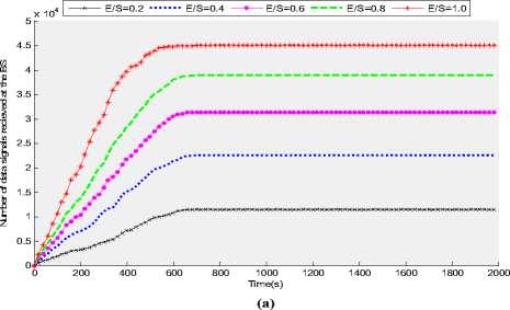
Figure 4: (a) Number of data signals received at the BS over time for different values of E/S (the ratio of event field area versus sensor field area) (b) Number of data signals received at the BS per given amount of energy for different values of E/S (the ratio of event field area versus sensor field area

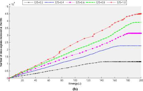
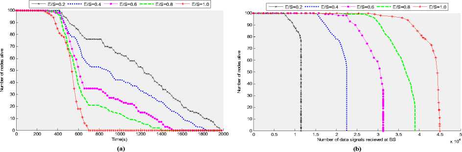
Figure 5: (a) Number of nodes alive over time for different values of E/S (the ratio of event field area versus sensor field area) (b) Number of nodes alive per amount of data sent to the BS for different values of E/S (the ratio of event field area versus sensor field area)

Ratio of EF area vs SF area                      Ratio of EF area vs SF area                      Ratio of EF area vs SF area                      Ratio of EF area vs SF area

(a)

(b)

(c)

(d)

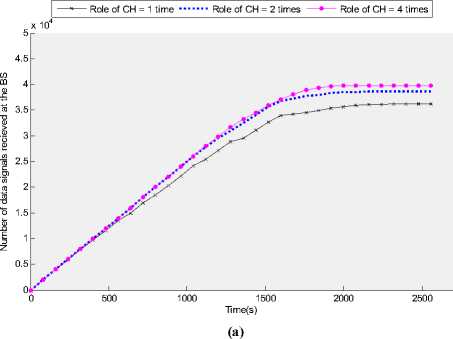
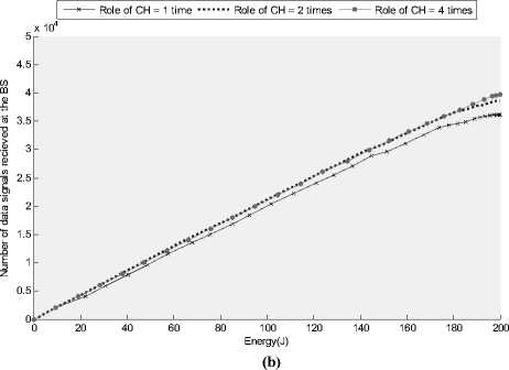
Figure 7: (a) Number of data signals received at the BS over time for different values of role of CH (b) Number of data signals received at the BS per given amount of energy for different values of role of CH

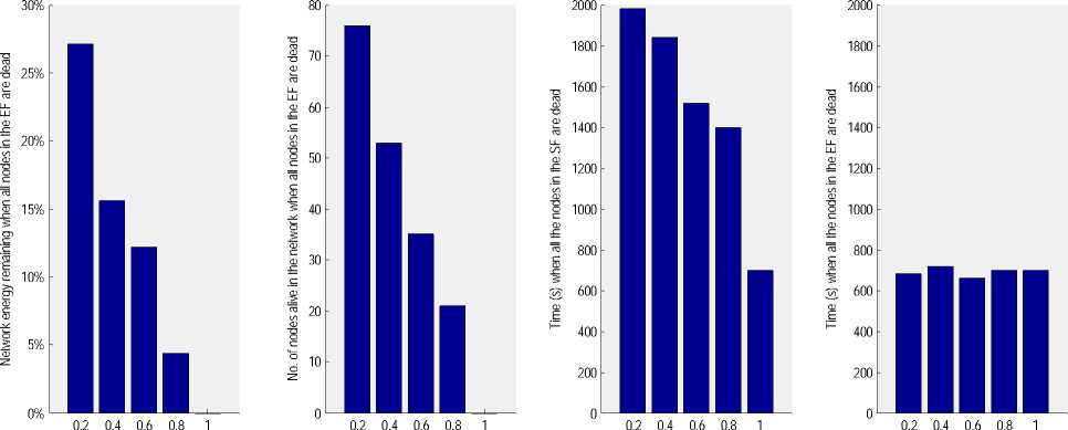
Figure 6: (a) Network energy remaining when all the nodes in the Event Field (EF) are dead for different values of E/S (the ratio of event field area versus sensor field area) (b) Number of nodes alive in the network when all the nodes in the Event Field (EF) are dead for different values of E/S (the ratio of event field area versus sensor field area)(c) Time (s) when all the nodes in the Sensor Field (SF) are dead for different values of E/S (the ratio of event field area versus sensor field area) (d) Time (s) when all the nodes in the Event Field (EF) are dead for different values of E/S (the ratio of event field area versus sensor field area)

Role of CH = 1 time Role of CH = 2 times Role of CH = 4 times

(a)

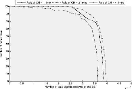
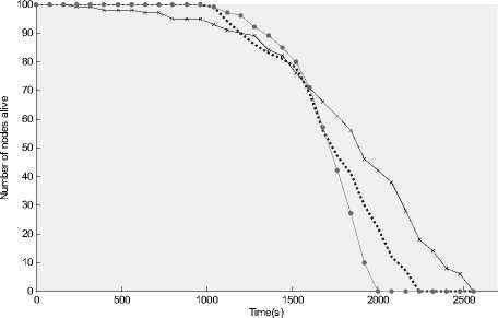
Figure 8: (a) Number of nodes alive over time for different values of role of CH (b) Number of nodes alive per amount of data sent to the BS

for different values of role of CH

Fig. 6 (a) shows the network energy remaining when all the nodes in the EF are dead for different values of E/S. This is the amount of energy for which not even a single communication activity will take place as all nodes that are alive are located outside the EF. Fig. 6 (b) shows the number of nodes alive in the network when all the nodes in the EF are dead for different values of E/S. As it was expected for smaller values of E/S, the number of nodes that are still alive is much higher as majority of the nodes are located outside the EF.

Fig. 6 (c) shows time in seconds when all the nodes in the SF are dead for different values of E/S. Looking at the graph of Fig. 6(c), initially it looks like that for smaller values of E/S, the overall network life time is increased. Fig. 6 (d) shows the time in seconds when all the nodes in the EF are dead for different values of E/S. This will be time from which onwards their will be no communication activity that will take place as all those nodes which can detect the event from within the EF are already dead. Interestingly the time value is same approximately for all the values of E/S. So if we define the network lifetime as time when all the nodes within the EF are dead (which is a more realistic definition) then using the LEACH protocol, we are not having an additional lifetime for smaller values of E/S even though still we have a lot of nodes that are still alive.

Fig. 7 (a) and (b) show the total number of effective data signals received at the BS over time and total effective data received at the BS for a given amount of energy respectively for different values of role of CH during the network lifetime. It is worth mentioning that more frequent repetition of the role of CH will induce an increased overhead that will be required due to control signal required for the formation of clusters during the cluster setup phase. Ideally a good clustering protocol should provide desired performance when role of CH value is set to one i.e. each sensor node is set to take the responsibility only once during the network lifetime. Fig. 7 (a) and (b) show that for smaller values of role of CH, lesser amount of data signals are received at the base