Performance analysis of convolution code with variable constraint length in shallow underwater acoustic communication

Автор: Krishnamoorthy Narasu Raghavan, Suriyakala C. D., Ramadevi Rathinasabapathy, Marshiana Devaerakkam, Sujatha Kumaran

Журнал: International Journal of Computer Network and Information Security @ijcnis

Статья в выпуске: 2 vol.11, 2019 года.

Бесплатный доступ

One of the most complex environment for the data transmission is the underwater channel. It suffers frequency selective deep fading with serious multi path time delay. The channel also has limited bandwidth. In this paper, the effect of Least Code Weight – Minimum Hamming Distance (LCW-MHD) polynomial code is studied using Viterbi Decoding Algorithm for the shallow Underwater Acoustic Communication (UAC) channel. Two different channels with the range of 100 and 1000 meters are considered for simulation purpose and the channel is designed using Ray Tracing algorithm. For data and image transmission in the channel, three different code rate of 1/2, 1/3 and 1/4 are considered and corresponding Bit Error Rate (BER) are evaluated. Result showed that the BER is least for the LCG-MHD polynomial code.

Еще

Viterbi decoding, Hamming distance, Underwater Acoustic Communication Channel, Ray Tracing, Ambient Noise

Короткий адрес: https://sciup.org/15015664

IDR: 15015664 | DOI: 10.5815/ijcnis.2019.02.02

Текст научной статьи Performance analysis of convolution code with variable constraint length in shallow underwater acoustic communication

Published Online February 2019 in MECS

In the recent years, different modes communication in UAC is investigated. In general, communication in UAC channel can be done by laser light or acoustic waves. High data rate and long range communication can be achieved using the laser light. But it suffers large attenuation and results in low BER [1, 2]. The major drawback is line of sight, failing results in the loss of communication. High speed, long-range underwater communication [3] is demonstrated using blue light with the wavelength of 405 nm. It is found that the laser diode with maximum output power is less absorbed in water and hence it provides a long range communication in underwater. For high speed communication authors make use the property of optoelectronic feedback and light injection technique. Authors showed that BER of 10-2 can be achieved without the equalizer and Low Noise Amplifier (LNA) and BER is improved to 10-4.

In [4], Optical wireless communication in UAC using Gallium Nitride (GaN) blue laser diode is demonstrated. The information is encoded using 490 nm Laser diode and modulated by 16 QAM. The encoded data is passed through a tank setup of 6.4 meters length. In the receiver section, authors used OFDM techniques along with QAM scheme for the detection of the data. They achieved a BER of 3.8x10-3 with the data rate of 8.8 Gbps at Average SNR (ASNR) of 16 dB.

To avoid the line of sight and ensure better perform in UAC channel, acoustic waves can be used instead of laser light. Acoustic waves are suffered by least attenuation since it uses low frequency. The desired BER can be achieved by proper coding techniques. In [5], the modeling of dynamic sea surface effects by wind generated waves and bubbles are carried out. It is based on the ray tracer together with a toolbox for generation of rough sea surface evolutions. Sea surface reflection loss is modeled with a modified sound profile in the frequency range of 1-4 kHz. They showed that in the frequency range of 4-8 kHz, the effects of the bubbles contributes significant additional effects on surface loss.

In [6], channel design using ray tracing techniques in temporal snapshots of an environment is demonstrated. For the given ocean condition and location of source and receiver, the impulse response of the channel is computed. It is also referred as the time arrival structure of the channel. The receiver is modeled by convolving the time arrival structure with the source data. Using ray tracing program, parameters such as amplitude, travel time and angle are computed.

In this paper, ray tracing technique is used to compute the impulse response of the channel, through which the various coding techniques are applied and BER is evaluated. LCG-MHD polynomial code is applied to the channel and BER is determined with the constraint length ranges from 1 to 3. The performance of the convolution code with the code rate of 1/2, 1/3 and 1/4 in the UAC is studied.

II. Related Works

The most effective and economical way of data transmission in the digital communication is the Forward Error Correction (FEC) coding. In this, the error can be detected and corrected in the receiver section. In [7], the non-uniform frequency offset created by the UAC is addressed. Maximum likelihood estimation is applied to estimate the Doppler shift and adaptive algorithm is used to correct the phase shift. Authors demonstrated the proposed algorithm in shallow water with a range of 1 km. They have achieved the error free communication in three different experimental setup using BCH (64, 10) code. In the first setup, four transmitters with 1024 carriers were used at 24 kHz bandwidth and able to achieve 18.9 kb/s data rate. In the second and third setup, they achieved a data rate of 26.8 kb/s and 2.1 kb/s using 2048 and 256 carrier respectively.

The Extrinsic Information Transfer Chart (EXIT) analysis using the Bit Interleaved Coded Modulation (BICM) and decision feedback equalizer in a UAC channel was performed in [8]. In the sea trial conducted by the author, the transmitter and receiver are separated by the distance of 200 meters with transmitter and receiver depth of 10 m and 5 m respectively. The input carrier frequency of 12 kHz was used with the bandwidth of 4 kHz. Convolution code with polynomial (23, 35) was used for the encoding purpose. The encoded data is modulated by BPSK with PN training sequence. For decoding of data, RLS algorithms with 30 taps were employed. The results showed that as the number of feedback tap increases the number of iteration decreases. It also evident that an error free communication can be achieved and BICM is depends on the number of taps in the equalizer and ISI in the channel. They also demonstrate that if the equalization is the success in the initial stage, then the receiver requires less iteration.

In [9], investigation of the application of the turbo equalizers in the UAC communication is carried out. The relation between the direct adaptive linear turbo equalizer (TEQ) and the MMSE turbo equalizer described. For encoding of data, Recursive Systematic Convolution (RSC) codes with random inter-leaver were used. The carrier frequency was set at 13 kHz and the decoding of data was done using turbo decoder with iteration value of 6. In a 1000 meter transmission range sea trial, the authors achieved a successfully decoding of the data with the data rate of 19.53 kbit/s. The need of energy and retransmission of the data in the FEC is greatly reduced.

But the complexity of the receiver is greatly increases as the constraint length increases.

In all the related study, the polynomial used in the convolution code has high code weight and hamming distance also maximum. By using LCW-MHD polynomial code in the convolution code, we can reduce the complexity of the receiver. In this paper, performance of the code is investigated for shallow water communication and its corresponding BER is evaluated.

To study the performance LCW-MHD code in the convolution code [10, 11], two different configurations are considered. The channel 1 has range of 100 meter whereas channel 2 has 1000 meters. Both the channels are having the Doppler shift of 3 x10^-4 Hz. Transducer and hydrophones are at a depth of 90 (Z s ) and 40 meters (Z) respectively. The other channel parameters are temperature = 10^oC, Salinity = 35%, PH = 8 ppt, wind speed = 23 knots and depth = 100 meters. To determine the losses in the channel. First Four Eigen rays [12, 13] are considered and are named as Direct Path (DP), Surface Reflected Path (SRP), Bottom Reflected Path (BRP) and Surface-Bottom Reflected path (SBRP). Their corresponding lengths and time taken to reach the receiver are calculated and listed in Table 1.

Table 1. Design Parameters for Channel 1 and 2

Parameters	Channel 1
Parameters	DP	SRP	BRP	SBRP
Distance travelled by the paths (in meters)	111	122	164	269
Time taken by the paths (in seconds)	0.074	0.081	0.109	0.179
Delay time with respect to DP	-	0.007	0.035	0.105
Overall Loss by the path (in dB)	92	97	142	149
Parameters	Channel 2
Parameters	DP	SRP	BRP	SBRP
Distance travelled by the paths (in meters)	1001	1002	1008	1030
Time taken by the paths (in seconds)	0.667	0.668	0.672	0.686
Delay time with respect to DP	-	0.001	0.005	0.019
Overall Loss by the path (dB)	96.5	101.5	131.5	136.5

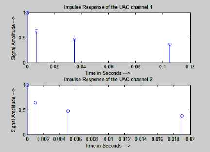
Fig.1. Impulse Response of UAC Channels

III. Proposed Convolution Code in UAC

The binary data can be encoded using convolutional codes in two different ways such as feed-forward and feedback. In the feed-forward type, the input data passes through a series of shift register and it is encoded using generator matrix. Whereas in the feedback type, a portion of output is given feedback to the input side and then encoded is done. An example for both feedback and feedforward shown in the Fig. 2 (a) and (b).

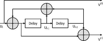
Fig.2 (a). Feedback Encoder

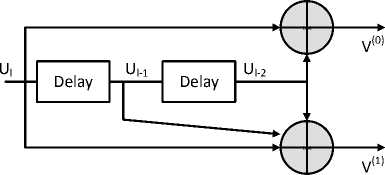
Fig.2 (b). Feed-Forward Encoder

Fig. 2 (a) shows the systematic feedback convolutional encoder and Fig. 2 (b) shows the non-systematic feedforward encoder for the same code rate of ½ with 2 memory element. The decoding of the convolution code is carried out by the Viterbi decoding algorithm in the receiver section after passing through the channel [22, 23]. In [24], authors explained a new way decoding the data using decode and forward delay protocol using Low Density Parity Check code. The general block diagram for the convolution code in UAC is shown in the Fig. 3. In the transmitting section, the binary data is encoded by the LCW-MHD code using convolution code and send it to the UAC channel . The original data is retrieved from the degraded data using the Viterbi algorithm in the receiving section. Finally the transmitted data is compared with the retrieved data and BER is computed. For each code rate, a memory element of 1, 2, and 3 is considered and BER is evaluated.

For simulation purpose, binary data of length 1000 is generated using the MATLAB function randint with the probability of zero as 0.5. The data is encoded using poly2trellis function and allowed to pass through the channel1 and 2. The encoded data size will be doubled for the code rate of 1/2 and three times the message for the code rate of 1/3 and four times for the code rate of 1/4. In the receiver side, the data from the channel is in complex form. To get back the binary data, the received data is quantized and given to the decoder. The Viterbi algorithm is applied in the decoder section to retrieve back the original data. While decoding, trace-back length of 8 is applied. BER is computed by comparing the decoding data with the original message bit.

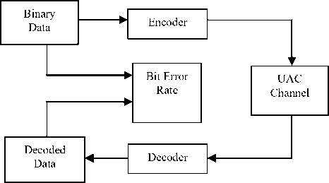
Fig.3. Block Diagram for Convolution Coding

3.1. Code rate of 1/2

For the code rate of 1/2 with constraint length of 1, input data is encoded with one shift register. Four codewords are possible in this case and they are named as 0, 1, 2 and 3. To encode the data, generator polynomials are formed using the adjacent code-word. The only adjacent polynomial is (1, 3). For Additive White Gaussian Noise (AWGN) channel, the code-word (1, 2) will give an optimal Bit Error Rate (BER). The error rate for this polynomial is compared with the adjacent polynomial (1, 3) for the channel 1 and 2 is listed in Table 2. It is observed that the polynomial (1, 3) performs well compared to the polynomial (1, 2).

Table 2. BER of UAC Channel for code rate of 1/2 with m = 1

Generator sequence (g⁰ g¹)	Code weight	Channel 1		Channel 2
Generator sequence (g⁰ g¹)	Code weight	Max BER	Min BER	Max BER	Min BER
(1, 2)	2	0.398	0.058	0.391	0.059
(1, 3)	3	0.269	0.036	0.313	0.037

For the code rate of 1/2 with constraint length of 2, the list of the polynomial for the generator matrix is listed in Table 3. The code-word of the polynomial is chosen in such a way that the code-words should have least code gain and minimum hamming distance. For example, the adjacent code-words for 1 are 3, 4 and 5. The set of polynomials are (1, 3), (1, 4) and (1, 5). Out of these, (1, 5) have a hamming distance of 1 whereas the other sets will have hamming distance as 2. So the polynomials (1, 5) are considered for evaluation purpose.

Similarly, for the code-word 3, the adjacent codewords are 1, 2, 5, 6 and 7. So the set of the polynomial are (1, 3), (2, 3), (3, 5), (3, 6) and (3, 7). Of these, polynomial set (3, 7) have the least hamming distance of 1. Other sets have hamming distance more than 1. The same procedure is done for all the code-word from 0 to 7 and the final list of the least adjacent polynomial for the code rate of 1/2 with 2 memory elements and its corresponding BER for the channel 1 and 2 are shown in Table 3. It is evident that the sequence with least code weight of 3 gives minimum BER than the sequence with code weight of 5.

The sequence (1, 5) gives a BER of 0.0348 then the sequence (5, 7) with BER value of 0.0696. It is concluded that the sequence (1, 5) perform well and gives the 50% less BER than the sequence (5, 7). The same procedure is repeated for the constraint length of 3. BER is calculated by varying the E b /N o value from 0 to 30.

Table 3. BER of UAC channel for code rate of ½ with m = 2

Generator sequence (g⁰ g¹)	Code weight	Channel 1		Channel 2
Generator sequence (g⁰ g¹)	Code weight	Max BER	Min BER	Max BER	Min BER
(1, 5)	3	0.280	0.034	0.283	0.035
(3, 7)	5	0.457	0.068	0.478	0.078
(4, 5)	3	0.291	0.036	0.316	0.039
(5, 7)	5	0.485	0.071	0.458	0.070
(6, 7)	5	0.467	0.062	0.424	0.061

The Table 4 shows the BER comparison of the channel 1 and 2 with the constraint length of 3. The maximum BER corresponds to the Eb/No value of 1 and minimum BER for the Eb/No value of 30. The result also showed that the as the code weight increases, BER also increases. For the code weight of 3 the BER is 0.04. The error rate is 0.06 and 0.07 for the code weight of 5 and 7. As the code weight doubles, the error rate also doubles. The sequence (13, 17) performs well in the AWGN channel, whereas in the case of UAC channel, the sequence (10, 11) with least code weight of 3 performs well then the sequence (13, 17). By comparing the Tables 2, 3 and 4, it is observed that as the constraint length increases, the error rate decreases slightly from 0.05 to 0.03.

Table 4. BER of UAC channel for code rate of ½ with m = 3

Generator sequence (g⁰ g¹)	Code weight	Channel 1		Channel 2
Generator sequence (g⁰ g¹)	Code weight	Max BER	Min BER	Max BER	Min BER
(10, 11)	3	0.371	0.050	0.333	0.040
(11, 13)	5	0.460	0.073	0.432	0.063
(12, 13)	5	0.464	0.066	0.463	0.073
(13, 17)	7	0.488	0.081	0.473	0.076
(14, 15)	5	0.468	0.068	0.473	0.076
(15, 17)	7	0.458	0.075	0.472	0.076
(16, 17)	7	0.459	0.073	0.482	0.080

3.2. Code rate of 1/3

For the code rate of 1/3 with the constraint length of 1, 2 and 3, the possible adjacent polynomial sequences are 2, 12 and 18. The BER values for this sequence are listed in

Table 5, 6 and 7 respectively. For m = 1, the code weights for the polynomial (1, 2, 3) and (1, 3, 3) are 4 and 5 and their corresponding error rate are 0.02 and 0.04. Similarly, for other two cases of m, the BER is increased more than doubled as the code weights are increased by two. In Table 6, the error rate for sequence (1, 4, 5) is 0.0258, whereas for the sequence (5, 7, 7) it is 0.0679. The code weights for this sequence are 4 and 8 respectively. For m = 3, the BER is 0.0284 for the sequence (10, 11, 14) and for the sequence (13, 15, 17) it is 0.05.

Table 5. BER of UAC channel for code rate of 1/3 with m = 1

Generator sequence (g⁰ g¹ g²)	Code weight	Channel 1		Channel 2
Generator sequence (g⁰ g¹ g²)	Code weight	Max BER	Min BER	Max BER	Min BER
(1, 2, 3)	4	0.303	0.035	0.222	0.025
(1, 3, 3)	5	0.346	0.041	0.374	0.048

Table 6. BER of UAC channel for code rate of 1/3 with m = 2

Generator sequence (g⁰ g¹ g²)	Code weight	Channel 1		Channel 2
Generator sequence (g⁰ g¹ g²)	Code weight	Max BER	Min BER	Max BER	Min BER
(1, 3, 5)	5	0.404	0.049	0.292	0.027
(1, 3, 7)	6	0.278	0.027	0.290	0.028
(1, 4, 5)	4	0.222	0.024	0.221	0.026
(1, 5, 7)	6	0.298	0.029	0.319	0.032
(2, 3, 6)	5	0.373	0.044	0.345	0.042
(2, 3, 7)	6	0.247	0.025	0.340	0.033
(2, 6, 7)	6	0.310	0.031	0.351	0.038
(3, 5, 7)	7	0.394	0.041	0.406	0.040
(3, 6, 7)	7	0.478	0.072	0.474	0.073
(4, 5, 7)	5	0.302	0.030	0.375	0.041
(5, 6, 7)	7	0.386	0.039	0.423	0.046
(5, 7, 7)	8	0.468	0.069	0.468	0.068

Table 7. BER of UAC channel for code rate of 1/3 with m = 3

Generator sequence (g⁰ g¹ g²)	Code weight	Channel 1		Channel 2
Generator sequence (g⁰ g¹ g²)	Code weight	Max BER	Min BER	Max BER	Min BER
(4, 14, 15)	6	0.305	0.031	0.341	0.036
(5, 14, 15)	7	0.472	0.068	0.437	0.052
(5, 15, 17)	9	0.487	0.067	0.447	0.054
(6, 16, 17)	9	0.464	0.059	0.489	0.067
(7, 15, 17)	10	0.463	0.056	0.449	0.052
(7, 16, 17)	10	0.478	0.075	0.478	0.079
(10, 11, 14)	5	0.378	0.030	0.443	0.028
(10, 11, 15)	6	0.313	0.038	0.322	0.032
(10, 14, 15)	6	0.433	0.068	0.303	0.050
(11, 13, 15)	8	0.475	0.067	0.443	0.059
(11, 13, 17)	9	0.411	0.044	0.437	0.048
(11, 14, 15)	7	0.476	0.054	0.455	0.055
(11, 15, 17)	9	0.408	0.043	0.428	0.049
(12, 13, 16)	8	0.423	0.044	0.368	0.036
(12, 13, 17)	9	0.424	0.045	0.426	0.452
(12, 16, 17)	9	0.457	0.059	0.452	0.050
(13, 15, 17)	10	0.457	0.053	0.466	0.059
(13, 16, 17)	10	0.484	0.059	0.444	0.051

3.3. Code rate of 1/4

For the code rate of 1/4 with the constraint length of 1, 2 and 3, the numbers of possible adjacent polynomial sequences are 1, 3 and 10. The BER values for this sequence are listed in Table 8, 9 and 10 respectively. For m=1, there is only one sequence of code weight 6 and its corresponding error rate 0.058. Similarly, for other two cases of m, the error is increased more than double as the code weights are increased by two. In Table 9, the error rate for sequence (2, 3, 6, 7) is 0.03, whereas for the sequence (5, 5, 7, 7) it is 0.06. The code weights for this sequence are 8 and 10 respectively. For m=3, the BER is 0.0183 for the sequence (2, 3, 12, 13) and for the sequence (13, 13, 15, 17) it is 0.03. The error rate starts decreases as the length of memory increases.

Table 8. BER of UAC channel for code rate of 1/4 with m = 1

Generator sequence (g⁰ g¹ g² g³)

Code weight

Channel 1

Channel 2

Max

BER

Min

BER

Max

BER

Min

BER

(1, 1, 3, 3)

0.383

0.051

0.419

0.058

Table 9. BER of UAC channel for code rate of 1/4 with m = 2

Generator sequence (g⁰ g¹ g² g³)	Code weight	Channel 1		Channel 2
Generator sequence (g⁰ g¹ g² g³)	Code weight	Max BER	Min BER	Max BER	Min BER
(1, 3, 5, 7)	8	0.355	0.036	0.418	0.048
(2, 3, 6, 7)	8	0.352	0.034	0.347	0.035
(5, 5, 7, 7)	10	0.452	0.063	0.456	0.062

Table 10. BER of UAC channel for code rate of 1/4 with m = 3

Generator sequence (g⁰ g¹ g² g³)	Code weight	Channel 1		Channel 2
Generator sequence (g⁰ g¹ g² g³)	Code weight	Max BER	Min BER	Max BER	Min BER
(1, 3, 11, 13)	8	0.330	0.027	0.375	0.037
(2, 3, 12, 13)	8	0.249	0.019	0.240	0.018
(4, 5, 14, 15)	8	0.328	0.029	0.373	0.037
(5, 7, 15, 17)	12	0.398	0.034	0.409	0.039
(6, 7, 16, 17)	12	0.480	0.058	0.462	0.056
(10, 11, 12, 13)	8	0.277	0.021	0.333	0.035
(11, 13, 15, 17)	12	0.389	0.033	0.441	0.043
(12, 13, 16, 17)	12	0.419	0.037	0.423	0.039
(13, 13, 15, 17)	13	0.371	0.030	0.367	0.030
(14, 15, 16, 17)	12	0.361	0.029	0.431	0.038

IV. Experiment Analysis

For image transmission in the UAC channel, a sample image is downloaded from google.com website. The input image is resized into 60 x 70 pixels and it is converted into its equivalent binary value. The size of the binary data has a length of 4200 bits. It is then encoded using the convolution code with a code rate of 1/2, 1/3 and 1/4 for three different constraint lengths of 1, 2 and 3. The encoded data is transmitted into to the UAC channel. The output from the UAC channel is decoded using the Viterbi algorithm with a trace-back value of 8. It is converted into integer value to get back the original image of size 60 x 70 pixel sizes. The decoded data is compared with the input data and BER value is determined. The Table 11, 12 and 13 shows the BER value for the different E b /N o value ranges from 5 to 30. It is evident from the Table 11 that the error rate is slightly decreases from 0.006 to 0.001 if the constraint length varies from 1 to 3.

For code rate of 1/3, the error rate is decreased rapidly from 1.15x10-4 to 5.77x10-5. Similarly, for the code rate of 1/4, the error rate is further decreased from 5.77 x10-5 to 8.6x10-6. It is concluded that for the image transmission in UAC channel, the error rate will be decreased drastically as the code rate and constraint length increases. Table 14 shows the minimum BER for the channel 1 and 2 for the Eb/No value of 30. For channel 1 and 2, the error rate is slightly increases from 0.03 to 0.05 for the code rate of 1/2.

Table 11. Image Transmission in the UAC Channel for code rate of ½

Generator sequence (g⁰ g¹)	E b /N o value
Generator sequence (g⁰ g¹)	5	10	20	30
(1, 3)			■ к
	0.4358	0.3460	0.1808	0.0060
(1, 2)
	0.3880	0.2610	0.1439	0.0012
(5, 7)	^^^^			;
	0.4792	0.4296	0.2248	0.0062
(1, 5)	Шй^й			- ' ' и'
	0.3355	0.3282	0.1588	0.0011
(13, 17)				^ ^^^
	0.4951	0.4474	0.2880	0.0033
(10,11)		■„: ■':'
	0.2928	0.2217	0.1107	0.0018

Table 12. Image Transmission in the UAC Channel for code rate of 1/3

Generator sequence (g⁰ g¹)		E b /N o value
Generator sequence (g⁰ g¹)	5	10	20	30
(1, 3, 3)	0.3234	0.1525	0.0508	8.371 x 10 4
(1, 2, 3)	0.4061	0.2924	0.1726	1.15 x 10^-4
(5, 7, 7)	0.4952	0.4579	0.2512	0.0617
(1, 4, 5)	'Я>^: 0.3459	0.1732	_V 0.0579	1.15 x 10^-4
(13, 15, 17)	0.49434	0.4714	0.1085	0.0015
(10,11, 14)	0.3583	веб 0.3011	0.465	5.77 x 10^-5

For code rate 1/3 the values are almost constant with 0.03 and for the code rate of 1/4 the BER value is decreased one fifth from 0.05 to 0.01. It is concluded that as the constraint length increases the error rate will be reduced. It also observed that the polynomial with least code weight performs well and gives minimum error rate than the polynomial with higher code weights.

Table 13. Image transmission in the UAC channel for code rate of ¼

Generator sequence (g⁰ g¹g² g³)	E b /N o value
Generator sequence (g⁰ g¹g² g³)	5	10	20	30
(5, 5, 7, 7)	■ 0.4724	0.4230	$^ж>Ж^ 0.2402	^ ^^^^ 0.005
(2, 3, 6, 7)	0.3393	0.2210	^ ^\| ^ 0.0370	^ ‘^ М' 5.77 x 10^-5
(13, 13, 15, 17)	0.4337	0.1390	0.0983	0.0022
(2, 3, 12, 13)	0.4674	0.4375	0.1065	8.66 x 10^-6

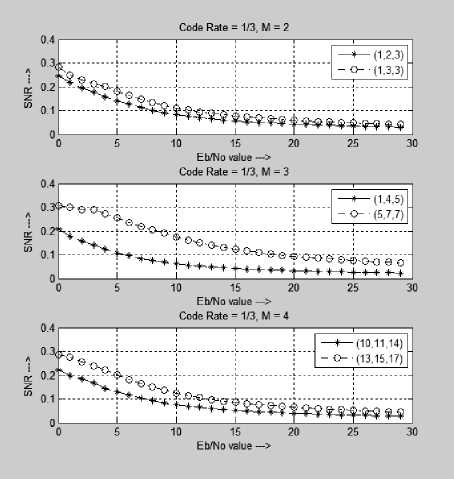
Fig.5. BER Comparison for the code rate 1/3

Table 14. BER Comparison for UAC channel with E b /No value of 30

Memory elements	Channel 1			Channel 2
Memory elements	Code rate 1/2	Code rate 1/3	Code rate 1/4	Code rate 1/2	Code rate 1/3	Code rate 1/4
M =1	0.036	0.035	0.051	0.037	0.025	0.058
M = 2	0.034	0.024	0.034	0.035	0.026	0.035
M = 3	0.050	0.030	0.019	0.040	0.028	0.018

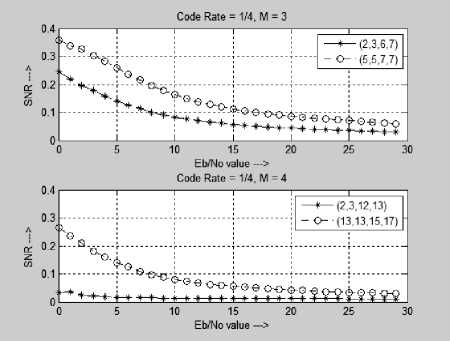
Fig.6. Comparison of the Generator Polynomial: code rate ¼

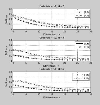
Fig.4. BER Comparison for the code rate ½

Fig. 4, 5 and 6 shows the BER comparison of the polynomial for the code rate of 1/2, 1/3 and 1/4 with a constraint length of 1, 2 and 3. The graph is simulated for the E b /N o value range from 1 to 30. The line with a circle is the optimal polynomial of AWGN channel and the line with asterisk * symbol is the polynomial with minimum code weight. It is clear observed that the polynomial which gives minimum error rate for AWGN is not the optimal polynomial for UAC channel. For code rate 1/2 and 1/3, as the constraint length increases, the BER is same. The error rate is reduced almost one fifth for the code rate of 1/4.

V. Conclusion

The performance of the convolution code in the underwater shallow communication is evaluated and analyzed. The BER in the order of 10-3 can be achieved for the code rate of 1/2. The BER can be further reduces in the order of 10-5 and 10-6 using the code rate of 1/3 and 1/4 with the memory element of 3. It is also observed that the polynomial with least code word and minimum hamming distance between the code word gives better BER than the other polynomial.

Список литературы Performance analysis of convolution code with variable constraint length in shallow underwater acoustic communication

J. Robert Urick, Principles of Underwater Sound for Engineers, McGraw-Hill, Third Edition, 2013.
A. Waite, Sonar for practicing Engineers, Wiley, Third Edition. 2005.
H. Chun Ming, L. Chang Kai, L. Hai Han, H. Sheng Jhe, C. Ming Te, Y. Zih Yi and L. Xin Yao, A 10/10 Gbps Underwater wireless laser transmission system, Optical Fiber Communications Conference and Exhibition (OFC), Los Angeles, USA, 2017, pp.1-3.
C. Yu Chieh, W. Tsai Chen, L. Che Yu, L. Hai Han, Hao K. Chung and L. Gong Ru, Underwater 6.4-m optical wireless communication with 8.8 Gbps encoded 480-nm GaN laser diode, International Semiconductor Laser Conference (ISLC), Hyogo, Japan, 2016, pp.1-2.
S. Henry Dol, Mathieu Colin, A. Michael Ainslie, A. Paul Vanwalree and Jeroen Janmaat, Simulation of an underwater acoustic communication channel characterized by wind generated surface waves and bubbles, IEEE Journal of Oceanic Engineering, Vol. 38, No. 4, pp. 642-654, October, 2013.
C. John Peterson, and B. Michael Porter, Ray/Beam tracing for modeling the effects of Ocean and platform dynamics, IEEE Journal of Oceanic Engineering, Vol. 38, No. 4, pp.655-665, October, 2013
C. Patricia Ceballos, and Milica Stojanovic, Adaptive channel estimation and data detection for underwater acoustic MIMO–OFDM systems, IEEE Journal of Oceanic Engineering, Vol. 35, No. 3, pp.635-646, July, 2010.
Shah, Charalampos C. Tsimenidis, Bayan Sharif and A. Jeffery Neasham, EXIT chart analysis of BICM-ID based receiver for shallow underwater acoustic communications, 7th International Symposium on Wireless Communication Systems, York, UK, 2010, pp. 6-10.
C. Jun Won, J. Thomas Riedl, Kyeongyeon Kim, Andrew C. Singer, and C. James Preisig, Practical application of turbo equalization to underwater acoustic communications, 7th International Symposium on Wireless Communication Systems, York, UK, 2010, pp. 601-605.
Elias Peter, Coding for noisy channels, IRE Conv. Rec., Part 4, pp. 37-47, 1955.
Massey, James, Threshold Decoding, MIT Press, Cambridge, Mass, 1963
B. Xu Zhi, and Y Lin Xue, Modeling Study of Hydro-acoustic Channel Based on Ray Model, Third International Conference on Information and Computing Wuxi, China, 2010, pp.217-220.
Chantri Polprasert, A. James Ritcey, and Milica Stojanovic, Capacity of OFDM systems over fading underwater acoustic channels, IEEE Journal of Oceanic Engineering, Vol. 36, No. 4, pp.514-524, October, 2011.
H. William Thorp, Deep-ocean sound attenuation in the sub and low kilocycle per second region, The Journal of the Acoustical Society of America, Vol. 38, No. 4, pp.648–654, July, 2005.
Fisher, and Simmons, Sound absorption in sea water, Journal of the Acoustical Society of America, Vol. 62, No. 3, pp. 864-875, June 1988.
Coates, An empirical formula for computing the Beckmann-Spizzichino surface reflection loss coefficient, IEEE Transactions on Ultrasonics, Ferroelectrics, and Frequency Control, Vol. 35, No. 4, pp. 522-523, July, 1998.
Alexios Korakas and Jens Martin Hovem, Comparison of modeling approaches to low frequency noise propagation in the ocean, MTS/IEEE OCEANS, Bergen, pp.1-7, October, 2013.
D. Adrian Jones, J. Alec Duncan, L. Amos Maggi, W. David Bartel, and Alex Zinoviev, A detailed comparison between a small-slope model of acoustical scattering from a rough sea surface and stochastic modeling of the coherent surface loss, IEEE Journal of Oceanic Engineering, Vol. 41, No. 3, pp.689-708, July, 2016.
L. Yu Kang and Yong Wang, Low-frequency sound transmission through water-air interface: A comparison between Ray and wave theory, OCEANS, TAIPEI, 2014, pp.1-5.
E. Lawrence Kinsler, R. Austin Frey, B. Alan Coppens and V. James Sanders, Fundamentals of Acoustics, Wiley, Third Edition, 1982.
S. Menonkattil Hariharan, Suraj Kamal and Saseendran Pillai, Reduction of self-noise effects in onboard acoustic receivers of vessels using spectral subtraction, Proceedings of the Acoustics Nantes Conference, Nantes, France, 2012, pp.3794-398.
J. Andrew Vitrebi, Error bounds for convolutional codes and an Asymptotically Optimum Decoding Algorithm, IEEE Transaction on Information Theory, IT-13, pp. 260-269, April, 1967.
G. David Forney, Convolutional Codes 1: Algebraic Structure, IEEE Transaction on Information Theory, 1970, pp. 720-738.
Jamaah Suud, Hushairi Zen, Al-Khalid B Hj Othman, Khairuddin Ab. Hamid, Decoding of Decode and Forward (DF) Relay Protocol using Min-Sum Based Low Density Parity Check (LDPC) System, International Journal of Communication Networks and Information Security, Vol. 10, No. 1, pp. 199-212, April 2018

Еще

Статья научная