Performance Analysis of Routing Protocols for Target Tracking in Wireless Sensor Networks

Published Online October 2016 in MECS DOI: 10.5815/ijmecs.2016.10.06

• I.    Introduction

  The various routing scheme either based on flat, hierarchical or geographical have been reviewed in the literature. These routing schemes employ some well-known data aggregation (Meng et al., 2013, Tharini et al., 2011) function at upper level to reduce number of messages for transmission to prolong the network lifetime. Some of the routing techniques are reviewed in Table 1.

Motivation: None of the existing routing protocols is suitable for target detection and tracking with. This motivate us to proposed a new hierarchical localization tracking scheme to improve messaging, network lifetime, reduce energy consumption, increase probability of target detection with good fault tolerance properties and scalability.

Contribution: We have proposed hierarchical target detection and tracking method for multiple moving targets at constant velocity. The target detected information is stored at node as well as two level of tree its parent and grandparent node. This increased small

Table 1. Routing Techniques in WSN

Algorithm	Routing technique
LEACH (Heinzelman et al., 2000)	Based on hierarchical topology with single hop. Selection of cluster head is based on some random probability threshold and it is rotational.
LEACH-F (Haas et al., 2002)	Fixed number of clustering based on hierarchical topology with single hop.
SPIN (Kulik et al., 2002)	Flat routing with multi hop. It is based on negotiation before data transmission. It used concept of ADV, REQ and DATA.
DD (Intanagonwiwat et al., 2005)	Routes are maintained as and when required, It is based on flat routing with multi hop. It used concept of interest and gradient.
EAR (Heinzelman et al., 2000)	Maintained several optimal path and selection is depends on probability of node energy consumption. Based on flat routing.

Redundancy but increase fault tolerance. This scheme reduces traffic implosion to log 2 N. Some of the basic challenges of routing and as well as target tracking for WSN are discussed below.

• A.    Energy Consumption

  Each sensor nodes have limited energy. Thus energy uses is very important for transmission of information in a multi hop wireless environment. Each node plays a multiple role as sender, receiver and router, so energy requirement is very crucial. Some sensor nodes dead due to power failure can cause significant network partition and reorganization network topology (Ian F. Akyildiz et al., 2004).

• B.    Scalability

Scalability measures the performance while number of sensor nodes increased. For large scale network, the number of sensor nodes deployed may be in the order of hundreds or even more. The network said to be scale if does not degrade its performance even for large number of sensor nodes (K. Akkaya et al., 2005).

• C.    Data Aggregation

  Sensor nodes usually sense similar information at multiple nodes at same duration. When same information is transmitted or forwarded towards the higher level nodes it is aggregated at some nodes (e.g. cluster heads) according to a certain data aggregation function, e.g., discarded suppression, count, summation, mean, minima and maxima (K. Khedo et al., 2010).

• D.    Connectivity

  The network connectivity is very important in sensor networks. If every sensor nodes reachable to other nodes in the network in any time, then network is always connected. Wireless ranges decide the connectivity of WSN (S. Gupta et al., 2011).

Section 2 makes review of the some existing routing protocols such as Sensor Protocols for Information via Negotiation (SPIN), Directed Diffusion (DD) and Low Energy Adaptive Clustering Hierarchy (LEACH) of different category. The survey motivates to move in the direction of proposing a hierarchical binary tree based scheme for target detection and tracking. Section 3 best describe the proposed HLTS scheme followed by section 4 of simulation environment. Section 5 elaborates the result for network life time, scalability, connectivity, energy consumption, probability of target detection and error rate following by conclusion in Section 6.

• II.    Routing Protocols for WSNs

  Routing protocols based on network structure is classified into two categories: flat routing and hierarchical routing. In a flat routing, all nodes are at same level with same functioning whereas in hierarchical routing they have different level with different functioning. We have reviewed some flat routing protocols Sensor Protocols for Information via Negotiation (SPIN) (Kulik et al., 2002), Directed Diffusion (DD) (Intanagonwiwat et al., 2005) and Energy-Aware Routing (EAR) etc. The typical hierarchical routing protocols in WSNs include Low-energy Adaptive Clustering Hierarchy (LEACH) (Heinzelman et al., 2000), Hybrid Energy-Efficient Distributed clustering (HEED) (Younis et al., 2004), Distributed Weight-based Energy-efficient Hierarchical Clustering protocol (DWEHC).

• A.    Sensor Protocols for Information via Negotiation

Sensor Protocols for Information via Negotiation (SPIN) is one of the flat routing protocols based on data centric negotiation. The SPIN protocol is designed to disseminate the data of individual nodes to all other sensor nodes. The main idea is to reduces duplicate information and prevent redundant data. For negotiation and data transmission, SPIN first uses ADV message to its neighbor nodes. Second message REQ is generate by the nodes those are interested. Third message DATA is send by the node to the requested neighbors (XuanTung Hoang et al., 2009). SPIN is event driven based negotiation. The data delivery ratio is lower but also has low routing overhead.

• B.    Directed Diffusion

Directed Diffusion ( DD) is categories as flat routing protocol which is data-centric protocol for dissemination. Directed diffusion is work in close proximity to localized the message exchanges within the limited network vicinity. The main parts of direct diffusion are request, message, reply and reinforcement. Directed diffusion is demand driven and it is improvement over SPIN using attribute-value pair. Direct diffusion has multiple paths, so data delivery ratio is higher than SPIN but suffer higher routing overhead.

• C.    Low Energy Adaptive Clustering Hierarchy

  Low-Energy Adaptive Clustering Hierarchy (LEACH) is the first clustering routing algorithms proposed for sensor networks and based on hierarchical routing. In a hierarchical routing, nodes are at different level with different group and according to level they have different tasks. The main tasks of LEACH are prolong network lifetime by reducing the number of transmission messages using data aggregation. LEACH partition the entire network into a set of cluster and each cluster has a randomly selected cluster head. All data aggregation is done by cluster head. Cluster head have sufficient energy for directly transfer data to base station. Once a node become a cluster head is no more allowed to become a cluster in any subsequent round. Each node has a time slot to transmit its data to cluster head using time division multiple access (TDMA) based schedule (Feng Wang et al., 2011)

• III.    Hierarchical Localization Tracking Scheme

The proposed Hierarchical Localization Tracking Scheme (HLTS) scheme is based on hierarchical tree. The scheme is for target tracking and localization, where sensor nodes are static and target are dynamic. This type of application required massive messaging for tracking of fast moving target. We have used concept of binary tree to store the sensed information at the node, parent and grandparent node of the sensor, which detect the target. The sensed information is further aggregate using some data aggregation technique such is minimum, mean and maxima and transmits to base station. The redundancy at two levels of trees improved the fault tolerance properties of the algorithm. This scheme reduces traffic implosion to log 2 N. We have used system model which includes:

Network model: We have considered a grid of square shape where k sensor nodes are placed randomly with density of λ using Poisson distribution as in (1) (Ahmed, T . et al., 2012)

P(N(A) =k) = ⁽ . е (1)

Where N (A) is the number of sensor nodes in area A. λ>0, is the average number of events per interval e is Euler’s number (e = 2.71828...) and k! is the factorial of k.

Target motion model: Assuming the target moves in a two-dimensional plane, the target motion model is described as in (2) (Chen et al., 2011).

X k+1 = F k X k +w k (2)

where X_k is the target state at the kth time stamp, F_k is the state transition matrix, and w_k ∼ N(0, Q_k) is the noise factor support Gaussian distribution and Q k is variance .

Define X k =[x k , x v , y k , y v ], where (x k , y k ) is the location of the target, and x v and y v are the target speed in x and y directions, respectively. Given the linear motion model, the next location of the target is given in (3) and (4).

x k+1 =x k +Т∗x v (3)

y k+1 =y k +Т∗y v (4)

Where T represents the sampling time and we used least square fitting method is used for target trajectory.

Target localization model: In general, a target can be detected by its nearby sensors. Therefore, we have used the simple centroid algorithm (Jie Li et al., 2015) to calculate the position of the target, which is described as in (5) and (6)

x t = ∑1=1 x i (5)

y t = ∑ill y t (6)

where ( X t ,У t ) is the estimated location of the target t, (( x i , y i ) is the location of sensor node s i detecting the target, and n is the number of sensor nodes detecting the target. This localization model is simple and works for all types of sensors.

In our proposed scheme we have used binary tree structure for positioning the nodes in the grid. As target object is sensed by the sensor nodes, than its parent and grandparent nodes are predicted to monitor the movements of the object. A target trajectory is computed using least square best fit method. Nodes tracking the object keep changing as the object moves and subsequent parent and grandparent nodes. The detection process is constantly track based on the location of the object at different time sampling at sequential time steps.

Algorithm- Target Detection

• 1.    Generate N number of the sensor nodes in area of A and they are placed randomly with density of λ using Poisson distribution.

• 2.    Target moves in two-dimension model using target motion model of equation (2).

• 3.    Compute the target location using centriod Algorithm as given in (4) and (5)

• 4.    Find the nearest sensor node‘s’, that detected the target‘t’ among all the nodes in that sensing range.

• 5.    Let sensor node‘s’, locate the target‘t’ and notify

• 6.    Repeat step 2 to 5 until all target located or Simulation time exhaust

• 7.    End Target Detection

its target prediction at its parent and grant parent node.

Path k [s] [t] [s] = 1

Path k [s/2] [t] [s] = 1

Path k [s/4] [t] [s] = 1

Algorithm: Target Trajectory (node)

• 1.    while (node !=NULL)

• 2.  { for i =1 to N do

• 3.    node =node->Lchild

• 4.  node = node->Rchild

• 5.  } /* end of while */

• 6.    Apply least square fit method for linear motion of target on all nodes on tracking path and also find fitting error

• 7.    Compute target detection probability with error

• 8.    end Target Trajectory

If Pathk [node] [t] [i] = 1 then store node i position in tracking path.

• IV. Simulation Environment

This section discusses the implementation specifics related to the simulation model and the various components of the simulation environment. It also provides descriptions of the various simulation parameters and analysis used in this study.

• A.    Performance Metric

We have measure performance analysis of our scheme with some existing method for the following performance metrics.

Network lifetime: The network lifetime is directly proportional to the number of live nodes in the network. Network lifetime is based on the ratio of dead nodes to the total number of nodes, focusing on the event-driven networks with Poisson model for packet generation. It is measure as number of rounds until simulation exhaust or network collapsed.

Routing Overhead: The routing overhead measures the total number of bytes sent as compared to actual data bytes sent. We have normalized routing overhead between 0 to 1 by scaling with number of bytes extra sent.

Scalability: A protocol is said to be scalable if it is perform well for large as well as small populations. A very crucial issue for WSN is the handling of a large number of nodes.

Average energy consumption: The average energy consumed by network is the total energy required by the nodes in sensing, receiving, forwarding, sleeping and transmitting the information. Initially each node assigned initial energy and its energy level is computed each time as per energy simulation parameters.

Target detection probability: Target detection probability measure how accurate the target detected. This required low false alarm rate and bounded detection delay. It is measure the sensing performance of the network.

Error rate: Number of times target wrongly detected.

• B.    Simulation Parameters

We have used following simulation parameters as mention in Table 2.

• V.    Results and Discussion

  Fig. 1 show the snapshot of nodes in the network where protocols are implemented. A 1000m*1000m square topology is considered and sensor nodes are placed using Poisson distribution with mean arrival rate is lambda. The base station, which is represented x, is located at the center of the network (500m, 500m). Here, the advance nodes having higher energy are shown by a plus symbol (+) and the normal nodes by a circle (0). In Fig. 1, 500 nodes are placed randomly in the network. Initially all nodes are live. The performance comparison is done in NS-2. Various performance metrics is computed to compare HLTS with the SPIN, DD and LEACH protocols.

• A.    Network Lifetime

Fig. 2 show performance graph between numbers of sensor nodes with network lifetime while transmission range is 100m.

Table 2. Simulation parameters

Simulation Parameter	Name/Value
MAC type	IEEE 802.11
Protocols	HLTS, DD, SPIN and LEACH
Application	Location estimation
Antenna type	Omni directional
Simulation duration	300 seconds
Terrain size (mxm)	500X500
Transmission range	100m to 400m
Sensing range	50m
Node speed	0 – 40 m/s
Number of sensors	50, 100, … 500
Packet size	512 bytes/packet
Transmit Power	360 mw
Propagation model	Two-ray ground reflection
Bandwidth	2 Mbps
Sensor radius (m)	50, 100, 150, 200
Channel type	Channel/ Wireless Channel
Interface queue type	Queue/Drop tail/ Priqueue

As number of sensor nodes increased, the network lifetime increases. The network lifetime is not well scalable for any of these protocols due to traffic implosion and geographical overlapping as network density increased. In this comparison network lifetime is measures as active number of nodes in the network. The HLTS has 10-20% higher network lifetime as compared to SPIN, LEACH and DD even when sensing range is higher. SPIN is worst hit as more messages generated for negotiations. SPIN and DD both not suitable for large scale network due to flat routing. LEACH and HLTS however have some scalable properties due to hierarchical properties.

Fig. 3 shows the comparisons between numbers of nodes vs. number of rounds. Increase in the network lifetime as number of nodes is increases. As number of nodes increases, more cover set generated. Thus excessive messaging is generated among the nodes. When number of nodes reached around 250-300 all protocols network lifetime (number of rounds) decreases due to higher network density.

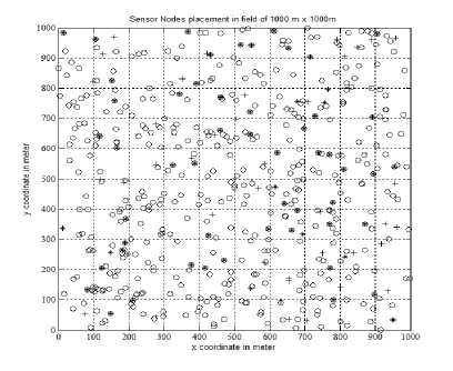
Fig.1. Sensor Nodes Distribution in 1000m x 1000m grid

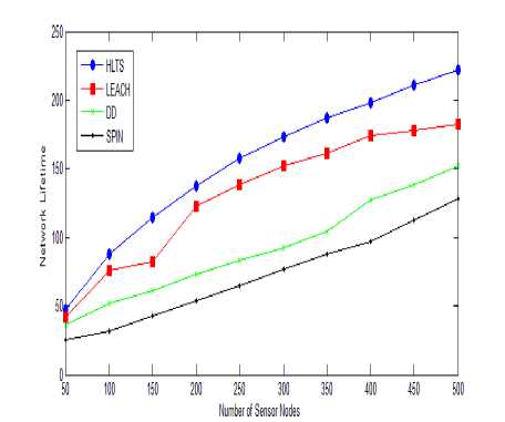
Fig.2. Number of Nodes vs. Network Lifetime

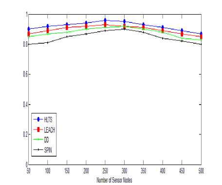
Fig.5. Data Delivery Ratio vs. Number of Nodes

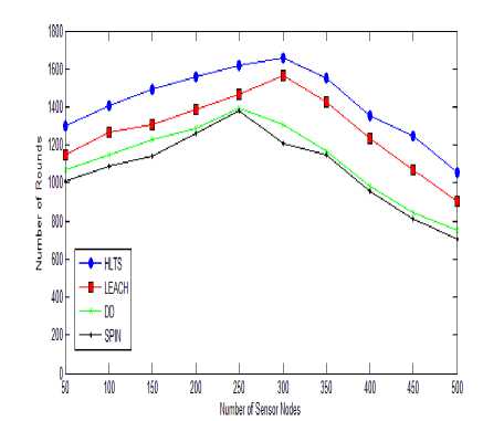
Fig.3. Number of Sensor Nodes vs. Number of Rounds

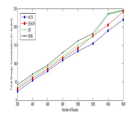
Fig.6. Total Energy Consumption vs. Number of Rounds

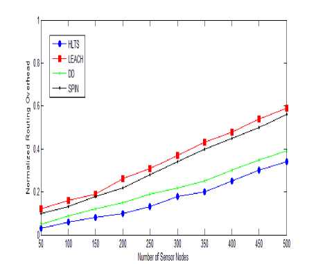
Fig.4. Normalized Routing Overhead vs. Number of Nodes

HLTS drops its number of rounds to 1100 when number of nodes reached 500. LEACH drops its number of rounds to 950 when number of nodes reached 500. DD drops its number of rounds to 850 when number of nodes reached 500. SPIN drops its number of rounds to 800 when number of nodes reached 500. Hence HLTS has 1520% higher network lifetime as compared to these protocols because HTLS maintained data at parent and grandparent node only in binary tree structure thus reducing the messaging to log2N.

• B.    Routing Overhead

Fig. 4 shows number of nodes vs. normalized routing overhead. When number of nodes around 100 in the network, the routing overhead is less for all protocols. As number of nodes increases routing overhead also increases. When number of nodes 500, SPIN protocols has 70% normalized routing overhead i.e. 70% extra bytes sent as compared payload. At the same scene HLTS has 38%, DD has 62% and LEACH has 45% normalized routing overhead.

As the number of nodes increased, normalized routing overhead increased sharply especially when number of nodes is high. DD suffer highest routing overhead as its nature is flooding and maintained multiple paths while leach has moderate routing overhead. HLTS has higher overhead but it is 20-30% less as compared to these two routing schemes. SPIN reduces the overhead as compared to DD. In SPIN a broadcast the metadata as an ADV message when it has data to send and waits for the request message REQ from the neighbor node and then send the DATA.

• C.    Scalability

The routing protocol is said well scaled when it experiences minimal performance degradation when used in increasingly large networks. Fig. 5 measure the scalability against the data delivery ratio by varying the number of nodes. HLTS, DD and LEACH routing scheme well scale up around 250- 300 nodes when network density is moderate. Packet delivery ratio more decreases for LEACH, SPIN and DD protocols as compared to proposed HLTS scheme while increasing the number of nodes to 500. Packet delivery ratio is 0.72 for SPIN, 0.73 for DD, 0.82 for LEACH and 0.9 for HLTS when nodes 500 in the network.

• D.    Total Energy Consumption

Fig. 6 shows the graph comparing the number of rounds vs. total energy consumption among SPIN, DD, LEACH and HLTS. In the proposed algorithm HLTS the total energy consumption is 95 Joules around at rounds 600, whereas SPIN protocol consumed 150 Joules, DD consumed 120 Joules and LEACH consumed 107 Joules with very good network lifetime. HLTS reduces energy consumption since only activated nodes in the network are involved in network and rest of nodes remains in sleep mode. Energy consumption increases for all routing scheme as number of nodes increase. But HLTS has 20% less consumption because its uses two level hierarchy of binary tree to store the redundant information.

• E.    Target Detection Probability

Fig. 7 shows the transmission range vs. probability of target detection. When a target is sensed by a sensor, a three dimension array is used to store the location of target. Xk store the target state at k step as well as the sensed node parent and grandparent node also store the target location. Target state is toggle between 0 and 1. When state is fixed i.e. either target is in or out from the trajectory. This is to minimizing false alarms. Up to transmission range 150m, all protocols have almost 90% target detection probability. As transmission range increases the target detection probability sharply decreases.

Fig. 8 shows the number of sensor nodes vs. probability of target detection with 100m transmission range and target velocity is constant of 10m/sec. As the number of nodes increasing all protocols have higher probability of target detection. Initially, as network density increased the connectivity as well as scalability also increased. As the number of nodes increases to high the performance of target detection draw back due to increasing network density. SPIN and DD protocols suffer very badly due to multiple copies of data is delivered. LEACH and HLTS both have limited traffic implosion but both affect from geographical overlapping due to increasing in network density. HLTS performance degrades by 10% whereas SPIN and DD suffer by 30%

Fig. 9 shows the target speed vs. probability of target detection with 100m transmission range and number of nodes 100. When target are static the probability of target detection is almost 90% for all four protocols. As the target speed increases the target detection probability decreases. SPIN and DD has 40% of target detection probability due to lots of multiple path generated due to fastest crossing of target to various sensor nodes.

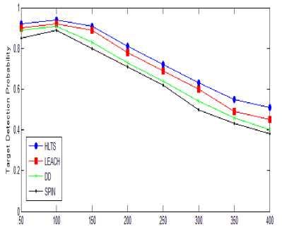
Transmission Range (m)

Fig.7. Transmission Range vs. Probability of Target Detection

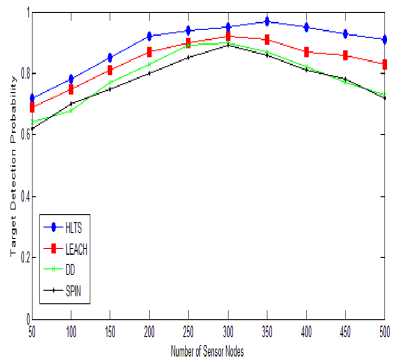
Fig.8. Number of Sensor Nodes vs. Probability of Target Detection

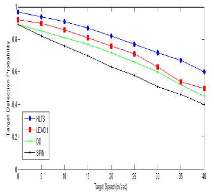
Fig.9. Target speed vs. Probability of Target Detection

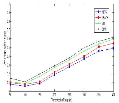
Fig.10. Transmission Range vs. Average Error Rate

HLTS also suffer with the same problem but it store sensed information at node, parent node and grandparent node only. Thus it performance degrade slowly to 60% at target speed 40m/sec. LEACH misses target almost 50% when target speed is 30 to 40 m/sec.

• F.    Error Rate

Average error rate are measure against the transmission range as shown in Fig. 10. Initially target state is toggle between 0 and 1 as the transmission range increases to 100. When state is fixed i.e. either target is in or out from the trajectory. This is to minimizing false alarms. Up to transmission range 150m, all protocols have almost 10% average error rate. As transmission range increases the error rate also sharply increases.

Fig. 11 shows the number of sensor nodes vs. average error rate with 100m transmission range and target velocity is constant of 10m/sec. When the number of nodes increasing error rate decreasing. Initially, as network density increased the connectivity as well as scalability also increased. As the number of nodes increases to 300 the error detection is only 5%. But as further increasing in number of nodes also increases network density as well as error rate. SPIN and DD protocols suffer very badly due to multiple copies of data is delivered. LEACH and HLTS both have limited traffic implosion but both affect from geographical overlapping due to increasing in network density. HLTS error rate is 12%, LEACH is 18%, DD is 22% and SPIN has 24%.

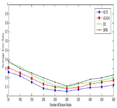
Fig.11. Target Speed vs. Average Error Rate

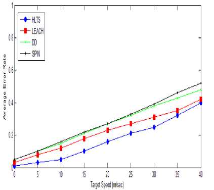
Fig.12. Target Speed vs. Average Error Rate

Average error rate are measure against the target speed in Fig. 12. As the target speed increases the error rate also increases for all the algorithms. When target are less mobile the error rate i.e. target not detected or wrongly detected or misplaced is 5% but when speed of target is 50 km/hour the error rate increase to 30%. At target speed 20m/s, average error rate for HLTS is only 5%, LEACH 8%, DD 10% and SPIN 18%. But as speed increased to 35m/s, average error rate for HLTS is only 10%, LEACH 30%, DD 33% and SPIN 45%. SPIN suffer badly due to excessive traffic implosion as target move with high speed more nodes generate excessive flooding.

• VI.    Conclusions

Simulation result proved that proposed HLTS scheme increases network lifetime by 25%, target detection probability by 25%, and reduces error rate by 20%, increased energy efficiency by 20%, fault tolerance, and routing efficiency. over the SPIN, DD and LEACH protocols. In future other hierarchical data structures like cube, hypercube, extended cube can also be studied for the target tracking