Performance Analysis of Texture Image Classification Using Wavelet Feature

Multi class image classification plays an important role in many computer vision applications such as biomedical image processing, automated visual inspection, content based image retrieval, and remote sensing applications. Image classification algorithms can be designed by finding essential features which have strong discriminating power, and training the classifier to classify the image. Scientists and practitioners have made great efforts in developing advanced classification approaches and techniques for improving classification accuracy [2,3,4,5,6 and 7].

In the past two decades, the wavelet transforms are being applied successfully in various applications, such as feature extraction and classification. Due to their scalespace localization properties, wavelet transforms (and their variants such as wavelet packets) have proven to be an appropriate starting point for classification, especially for texture images [8, 9]. Also the choice of filters in the wavelet transform plays an important role in extracting the features of texture images [8, 9].

In the work [10] describes multi spectral classification of land-sat images using neural networks. [11] Describes the classification of multi spectral remote sensing data using a back propagation neural network. A comparison to conventional supervised classification by using minimal training set in Artificial Neural Network is given in [12]. Remotely sensed data by using Artificial Neural Network based have been classified in [13] on software package. In [14] different types of noise are classified using feed forward neural network.

Naive Bayes [14, 15, 16] is one of the simplest density estimation methods from which a classification process can be constructed. KNN [17, 18] classification method is a simplest technique conceptually and computationally, but it still provides good classification accuracy. The KNN classification is based on a majority vote of k -nearest neighbor classes.

The drawback of multi-layer feed forward networks using error back propagation is that the best number of hidden layers and units varies from task to task and these are determined experimentally. If large number of hidden units are used then the network will learn irrelevant details in the training set. Similarly, if a network is very small, it will not be able to learn the training set properly. One approach to automatically determine a good size for a network is to start with a minimal network and then add hidden units and connections as required like the Cascaded Neural Networks. Cascade Feed Forward Neural Networks [19] helps in overcoming this shortcoming by increasing the number of hidden layers dynamically during the learning phase.

This paper is organized into mainly three sections. In the second section classifier used for performance analysis are discussed. Basically the performance is evaluated in four different classifiers as Naïve Bays Classifier, K-Nearest Neighbor (K-NN), Feed Forward Back Propagation Neural Network (BPNN) and Cascaded Neural Network. The third section presents the feature extraction algorithm as well as experimental results,

• II.    CLASSIFIERS

Image classification is also very important area in the field of computer vision, in which algorithms are used to map sets of input, attributes or variables – a feature space X - to set of labeled classes Y. Such algorithms are called as classifiers. Basically a classifier assigns a pre-defined class label to a sample. Fig 1 shows as simple architecture of the classification system. Any classification system has two stages, training stage and testing stage. Training is the process of defining criteria by which features are recognized. In this process the classifier learns its own classification rules from a training set. In the testing stage, the feature vectors of a query/test image works as input. A classifier decides on the bases of learning model, with its own classification rules, as to which class that feature vector belongs.

• A.    Naive Bayes Classifier

This is the simplest density estimation method which is used for classification process [14, 15, 16]. A Naive Bayes classifier categorize patterns to the class C to which it is most likely to belong based on prior knowledge.

Given a set of feature vectors = {^ , X2,…,X_n } and set of classes C ={ C*i , C2,.., Cm }

The corresponding classifier is the equation defined as follows:

C( Xi , x2,.,xn)= argmax p ( Cj)∏^iP( Xi │ C,)                     (1)

• B.    K-Nearest Neighbor

KNN [17, 18] classification method is a simplest technique conceptually and computationally, but it still provides good classification accuracy. The KNN classification is based on a majority vote of k-nearest neighbor classes. KNN classifier takes only k-nearest neighbor classes. So that majority vote is then taken to predict the best-fit class for a point. That means, in a k= 5 nearest neighbor classifier, the algorithm will take majority vote of its 5 nearest neighbors. For example, consider Fig 2(a) where k = 1, the feature vectors of query image, point X, belongs to class 3 (green circles). If k= 5 as in Fig. 2(b) the point X best-fit in class 1 (blue circles) according to majority vote of the five nearest points.

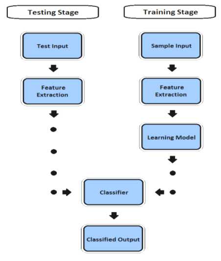
Figure:1. Design of classification system

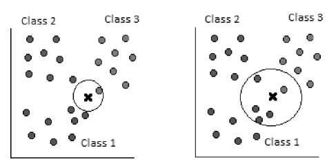
(a) 1-NN Classifier

(b) 5-NN Classifier

Figure 2: k -Nearest Neighbor classification

The Euclidean distance is used for measuring the distance between the test point and cases from the example classes. The Euclidean distance between two points, r and s, is the length of the line segment rs. Cartesian coordinates if r = (r_t,r2,…r ) and s = (s_t,s2,…․ѕ ,) are two points in Euclidean n- space, then the distance from r to s is given by:

d ( r , S )=√(r1 -ѕ1)2+(r2 -ѕ2)⁵+⋯+(r -ѕ ⁾²

=√∑ U (r -ѕ)²                     (2)

In image classification, Cheng et al. [20] used KNN classifier for 20 categories: firstly, images are segmented based on color and texture features. Yanai [21] classified color features into 50 conceptual categories using KNN classifier. Vogel et al. [22] used a KNN classifier to assign concept keywords to the different area of an image.

• C.    Feed Forward BPNN

Back propagation is a multi-layer feed forward, supervised learning network based on gradient descent learning rule. This BPNN provides a computationally efficient method for changing the weights in feed forward network, with differentiable activation function units, to learn a training set of input-output data. Being a gradient descent method it minimizes the total squared error of the output computed by the net. The aim is to train the network to achieve a balance between the ability to respond correctly to the input patterns that are used for training and the ability to provide good response to the input that are similar. A typical back propagation network of input layer, one hidden layer and output layer is shown in fig. 3.

The steps in the BPN training algorithm are:

Step 1: Initialize the weights.

Step 2: While stopping condition is false, execute step 3 to 10.

Step 3: For each training pair x:t, do steps 4 to 9.

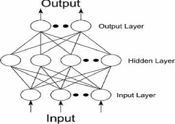
Fig 3: Feed Forward BPN

Step 4: Each input unit ,  =1,2,…, receives the input signal, xi and broadcasts it to the next layer.

Step 5: For each hidden layer neuron denoted as ,   =1,2,…․, .

z inj = ^Voj + S x i v ij

i

zj = f(zinj >

Broadcast to the next layer. Where v oj bias on j^th hidden unit.

Step 6: For each output neuron Y , k=1,2,…․m

Y ink = w ok + E z j w jk j

Y k = ^f( Y ink )

is the

Step 7: Compute 5_k for each output neuron, Y_k

'

⁵ k = ^(tk - Y k^)f (Y ink )

Awjk = a5 kZj

Awok = a5k    sin ce Zo = 1

Where ^ is the portion of error correction weight adjustment for w jk i.e. due to an error at the output unit y k , which is back propagated to the hidden unit that feed it into the unit y k and a is learning rate.

Step 8: For each hidden neuron

m

5inj =S5kwjk  j = 1,2.....p k=1

5 j =5 inj f'(Z inj )

A v ij = a5 j X i

Avoj = a5 j

Where A y is the portion of error correction weight adjustment for v ij i.e. due to the back propagation of error to the hidden unit z j

Step 9: Update weights.

w jk (new) = Wjk (old) + Aw jkVij (new) = Vj (old) + AVij

Step 10: Test for stopping condition.

• D.    Cascaded Neural Network

Cascaded Forward neural network system is similar to feed-forward networks, but include a weight connection from the input to each layer and from each layer to the successive layers. This also is similar to feed forward back propagation neural network in using the back propagation algorithm for weights updating, but the main symptom of this network is that each layer of neurons related to all previous layer of neurons [23].

• III.    RELATED WORK

This work is extension of the work [1] where the texture images of fifteen categories are classified using feed forward back propagation neural network. The performance of the system [1] is compared under four different classifier namely Naïve Bays, Cascaded Neural Network, K-Nearest Neighbor and Feed Forward Neural Network. Here the features are extracted from the texture images and these are applied to each of the classifier to train. Then features of the query images are extracted and applied to each classifier to test.

• A.    Computation of Feature

To assess the capability of wavelet feature based classification of images we have taken the texture images as shown in the fig. 4 from the database available by the University of Southern California’s Signal and Image Processing Institute Volume 1[24]. Features are extracted from the cumulative histogram of various combinations of the Haar wavelet coefficients of the original and complemented image [1]. This algorithm produces a vector of 384 descriptors. Every gray scale image is resized to 256x256, then it is divided into 64 blocks.

Then feature extraction algorithm [1] is applied to each of the block to create a feature database. Eight feature vectors of each image is used to learn the classifier, remaining are used to test.

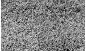
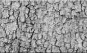
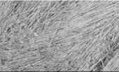
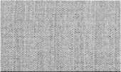
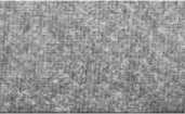
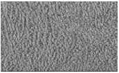
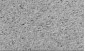
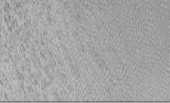
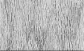
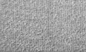
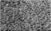
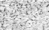
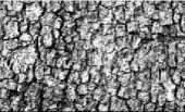
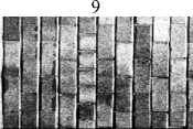
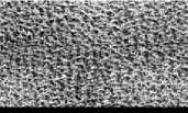
Figure.4: Texture Image from Brodatz album

Table I. Performance Evaluation

S.No .	Texture Image	Naïve Bays	Feed Forward BPNN	K-Nearest Neighbor	Cascaded Forward NN
1	Grass (D9)	82.81	91.56	75.5	89.25
2	Bark (D12)	70.31	92.25	61	75.6
3	Straw (D15)	53.12	82.12	61	74.23
4	Herring bone weave (D15)	71.89	86.02	79.7	91.29
5	Woolen cloth (D19)	53.12	95.6	68.6	83.54
6	Pressed calf leather (D24)	98.44	100	96.9	97.51
7	Beach sand (D29)	60	85.48	74.06	80.52
8	Water (D38)	96.87	100	98.5	94.3
9	Wood grain (D68)	55.29	93.54	82.9	70.48
10	Raffia (D84)	84.37	96.8	100	93.6
11	Plastic bubbles( D112)	85.93	86.4	80	88.3
12	Gravel	92.18	99.06	95.31	87.85
13	Field Stone	75	85.25	70.31	73.5
14	Brick wall	63.25	83.27	61.5	79.45
15	Pigskin (D92 H.E.)	61	91.56	84.37	83.54

Step 1 :Read the RGB image f(x, y, z)

Step 2:Convert the image to gray scale image f fry)-

Step 4:For each pair of coefficients (A,H),(A,V), (A,D) and (A-abs(V-H-D)) repeat the step5 to step8.

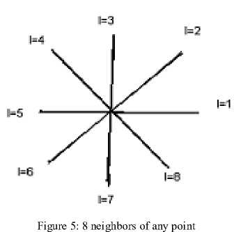
Step 5: For I=1 to 8 repeat the step 6 . Where I represents the 8 neighbors in each direction of any point as shown in fig. 2.

Step 6: Repeat for J=1 to M

Repeat for K=1 to N d=max(min(X(J,K),Y(I)),min(Y(J,K),X(I)))

if d=min(X(J,K))

Set H1(I)=X(J,K)

Else

Set H2(I)=Y(J,K)

End

End

Step 8:For each cumulative histogram correlation coefficient, mean and standard deviation features are computed.

• B.    Experimental Result and Discussion

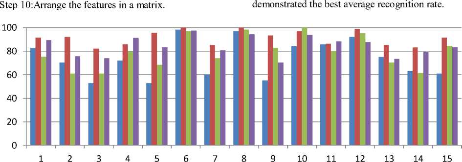
The classifiers are tested with the texture block of size 16x16. The experimental results of the proposed algorithm [1] of different texture images are compared in the Table.1, which shows the percentage classification rate for different image classes. The analysis of the experimental result shows that , in general, classification accuracy 73.57% is achieved by Naïve Bays classifier, 91.26% is achieved by Feed Forward Neural Network, 79.31% is achieved by K-Nearest Neighbor and 84.19% is achieved by Cascaded forward Neural Network.

Step 9:Repeat step3 to step 8 for complement image of f(x,y) also.

Fig. 6 showing experimental results using bar chart, which shows that Feed Forward Neural Network

Naïve Bays     Feed Forward BPNN     K-Nearest Neighbor     Cascaded Forward NN

• Figure 6: Comparison of recognition rate of classifiers

IV.CONCLUSION

In this paper a multi class texture images classification, using wavelet based features obtained from image and its complement image is presented. The experimental results are compared under four different classifier namely Naïve Bays, Feed Forward Back Propagation, K-Nearest Neighbor and Cascaded Forward Neural Network. The experimental results demonstrate the efficiency of the various classifiers for multiclass texture image classification. The results are encouraging.