Performance Evaluation of Distributed Protocols Using Different Levels of Heterogeneity Models in Wireless Sensor Networks

Published Online December 2014 in MECS DOI: 10.5815/ijcnis.2015.01.06

A wireless sensor network (WSN) consists of low-size and low-complex devices, which are called as sensor nodes. A sensor can sense the environment to gather information from the monitoring field and communicate through wireless links. The data collected by a sensor is forwarded via multiple hops to a particular node, called as a sink. The sink can utilize the received data or it can forward to other networks connected through internet. A sensor node can be in one of the states: stationary or moving. It may or may not have information about its location. The network can be homogeneous or heterogeneous. In a homogeneous network, all sensor nodes have the same amount of energy. A non-homogeneous network is called heterogeneous network. A WSN can be used in several applications such as national security, military, healthcare, environmental monitoring, temperature, humidity, vehicular movement, pressure, soil makeup, noise levels, presence or absence of certain types of objects [3]. Sensor network applications can be divided into two groups: querying applications and tasking applications. In querying applications, the information collected by sensors is processed based on the query that triggers the data collection action; for example, collecting the data about an event in the monitoring environment. In tasking applications, the data collection is triggered by an event that is to be observed by the network. An event triggering forces the sensor node to perform some action. The data aggregation is done in order to avoid duplication of data as the adjacent nodes may send some identical data to sink. Sensors can also be coordinated to get a better idea about the event; for example, some sensors can be moved closer to the event.

One of the most important features of a sensor network is its network lifetime. For enhancing the network lifetime, there have been discussed some protocols that include ALBPS and ADEEPS. These protocols assume the network to be homogenous. In ALBPS, the network is kept alive as long as possible by means of load-balancing. In ADEEPS, a low energy sensor tries to minimize its energy consumption rate for targets while allowing higher energy consumption for sensors with higher energy. The network lifetime can be increased by power saving techniques. These techniques may be classified in two categories: scheduling the sensor nodes to alternate between active and sleep mode, and adjusting the sensing range in wireless sensor nodes. Placing few heterogeneous nodes in the sensor network can bring the following three main benefits [6]: prolonging network lifetime, improving reliability of data transmission and decreasing latency of data transportation.

In this work, we concentrate on maximizing sensor network lifetime by using ALBPS and ADEEPS algorithms incorporated with different level of energy heterogeneity in sensor nodes. We make comparative analysis of homogeneous and heterogeneous versions of ALBPS and ADEEPS protocols. In this work, we use 2-level, 3-level and multi-level heterogeneity. The heterogeneous versions of ALBPS and ADEEPS have better performance than their homogeneous versions. Moreover, as the level of heterogeneity increases, the lifetime of the network also increases.

The rest of the paper is organized as follows. Section II discusses the literature survey. The proposed work is discussed in Section III and the simulation results are presented in section IV. Finally the paper is concluded in Section V.

• II.    Literature survey

In this section, we review the related existing works on improving the lifetime of wireless sensor networks. We consider three aspects in reference to improving the lifetime of WSNs that include scheduling algorithms, adjusting sensing range and heterogeneity of sensors.

In [1], Berman et al. discuss centralized and distributed algorithms for increasing the lifetime of sensor networks. These algorithms solve the area coverage problem and SNLP (Sensor Network Lifetime Problem). They use scheduling approach of sensor nodes and a method for solving the fixed range maximum lifetime problem. In this method, the sensing range cannot be changed and it is meant for homogeneous WSNs. Cardei et al. discuss another approach to extend the sensor network lifetime by organizing the Sensors into a maximal number of set covers that are activated successively. Only the sensors from the current active set are responsible for monitoring all targets. In their work they have provided the solution of the maximum set covers (MSC) problem and designed two heuristics to efficiently compute the cover sets [2]. In [4], Brinza and Zelikovsky discuss two distributed target monitoring protocols, namely Load-Balancing Protocol and DEEPS Protocol for lifetime problem. These protocols solve the target coverage problem by scheduling and fixed sensing range approach. Their work is an extension of distributed algorithm, discuss in [1]. Cardei et al. [3] address the target coverage problem with scheduling model and adjustable sensing range. In that work, adjustable range set covers (AR-SC) problem is solved by finding a maximum number of set covers and the ranges associated with each sensor in such a way that each sensor set covers all targets. A sensor can participate in multiple sensor cover sets. Dhawan et al. improve the lifetime of WSNs using both scheduling and adjusting sensing ranges. They discuss two completely localized and distributed scheduling algorithms such as ALBPS and ADEEPS with adjustable sensing range for coverage problem [5]. These algorithms may be considered as an enhancement of distributed algorithms for fixed sensing range discussed in [4].

Besides the scheduling and the adjustable sensing range in our work, we consider the heterogeneous energy levels such as 2-Level, 3- Level and multi-Level in sensor network [6-15]. We consider two scenarios that are for load balancing protocol and deterministic energy efficient protocol for WSNs. In both the scenarios the lifetime of the sensor network increases significantly using 2-level, 3-level and multilevel heterogeneity. As the level of heterogeneity increases, the lifetime of a WSN also increases. In the next section we discuss our proposed work.

• III.    Proposed work

Our proposed work is based on the ALBPS and ADEEPS protocols. These protocols consider three states for a sensor i.e, a sensor node can be in one of the three states: active, idle and deciding. In active state a sensor monitors the targets and in the idle / sleep state it conserves the energy. In the deciding state, it monitors targets and can change its current state. In ALBPS, a sensor in the deciding state with range r changes its current state to either active or idle state depending on its energy level for load balancing. It is also possible that it may not change its current state until the target is covered by any other active sensor node. In ADEEPS, there must be at least one sensor in-charge of each target. When a sensor is in the deciding state with range r, it changes its current state to either active or idle state. Whenever a sensor is not in-charge of any target, it switches to idle state [4]. An active sensor stays in that state for a certain period of time called shuffle time. In order to find its cover schedule, each sensor initially broadcasts its current energy level and covered targets to all neighbors, and then changes its current state to the deciding state with its maximum sensing range. During the shuffle time the active sensors update their energy levels.

We extend ALBPS and ADEEPS protocols by incorporating heterogeneity of various levels. The heterogeneity levels that are considered include 2-level, 3-level and multi-level heterogeneity. In these levels, the sensor nodes have different amounts of energy. In 2-level heterogeneity there are two types of sensor nodes and in 3-level there are three types of sensor nodes. In multilevel heterogeneity the energy is randomly distributed from a given energy interval to sensor nodes. Details of these levels of heterogeneity are given below.

• A.    2-Level Heterogeneity

In 2-level heterogeneity, there are two types of sensor nodes: advanced and normal nodes. Consider N sensor nodes that are deployed in a given rectangular area. Let E 0 be the initial energy of a normal node and m be the fraction of the advanced nodes, which own a times more energy than the normal ones. Thus there are m * N advanced nodes equipped with initial energy of Eо∗ (1 + a), and (1 - m) ∗ N normal nodes equipped with initial energy of E₀. The total energy for 2-level heterogeneity, denoted by E 2total , of the network [8] is given by

E 2 to tai = Ν ∗ (1 - m) ∗ EО+ Ν∗m∗ЕО ∗ (1 + a) =Ν∗ EО ∗ (1 + am) (1)

• B.    3-level Heterogeneity

In 3-level heterogeneity, there are three types of sensor nodes: super, advanced and normal nodes. Consider m fraction of N as advance nodes and m0 fraction of the advance nodes as super nodes. The normal nodes have E0 as initial energy. The energies of advance and super nodes are respectively and β times more than that of the normal nodes. Thus energies of the each super and advanced nodes are E о ∗ (1 + β) and Eо ∗ (1 + a) respectively. The total energy for 3-level heterogeneity, denoted by E3total, of the networks [6,7] is given by

Estotai = N * (1 - m) * E0 + N * m * (1 - m0) * E0

* (1 + a) + N * m * m0 * Eo * (1 + в)

E з to tai = N * Eo * (1 + m * (a + m0 * в))          (2)

• C.    Multi-Level Heterogeneity

In multi-level heterogeneity, the initial energy of sensor nodes is randomly allocated from the given energy interval [E_o , E_o * (1 + a_max)], where E₀ is the lower bound of the energy interval and a max determines the upper bound of the energy interval. Initially, the node s i is equipped with the initial energy of E_o * (1 + a , ), which is a_i times more energy than the lower bound E₀ of the energy interval. The total initial energy of the network with multi-level heterogeneity [8], denoted by E_mtotai, is given by

N

Emtotai = ^Eo* (1+ a I)

= E01* (N+ Z^ ,a,)         (3)

We now discuss our proposed work. In 2-level heterogeneity, initially the advance nodes are active nodes and they monitor the targets. If any target is not covered by the advanced nodes then some of the normal nodes that can monitor uncovered targets become active nodes. When during the reshuffle time the energy level of the active nodes becomes less than that of the normal nodes, then some of the normal nodes that can cover all targets become active.

In 3-level heterogeneity, initially the super nodes are active nodes and they cover the targets. In case some target is not covered by the super nodes, then some of the advance nodes that can monitor uncovered targets become active nodes. If some targets are still not covered by super/advance nodes, then some of the normal nodes that can monitor the uncovered targets become active nodes. When during the reshuffle time the energy level of the active nodes becomes less than that of the advance nodes (in case there are not active nodes) or normal nodes (which are not active nodes). These active nodes are replaced by the advance nodes. When the energy level of the active nodes becomes less than that of the super nodes (in active) or advanced nodes or normal nodes (in this order) then some of the super/advanced/normal nodes that can cover all targets become active nodes.

In Multi-level heterogeneity, initially the highest energy level nodes are active that cover all targets. If some targets are not coved by the highest energy level nodes, the nodes having less energy than the highest energy nodes that can cover the remaining targets become active. This process continues in a similar way as discuss for 3-level heterogeneity.

Here, we determine the cover sets by using the active nodes. The number of cover sets depend on the number of targets, sensor and target positions. We try to have minimum number of active sensors for monitoring all targets in a cover set so that minimum energy is used to monitor all targets. Other sensors become idle (go to idle states). Each active sensor broadcasts its covered targets, energy level and information about the change of states. If an active sensor nearly exhausts its energy supply and is going to die (Etotal = 0), it informs its neighbors about its energy level. A subset of neighbors which are in idle state changes to active states by replacing the exhausted sensor.

The proposed work consists of two algorithms which are based on load balancing and energy efficiency using set target in-charge. Their steps are given as follows:

Step1: Information about the sensor nodes and targets are stored in two vectors denoting as vectors i> and j> for sensor S_i and target Tj, respectively. The vector i> contains node id, total energy and x, y position of i^th sensor. The vector j> contains target id and x, y coordinates of j^th target.

Step2: Total energy of the network for 2-level, 3-level and multi-level heterogeneity is computed using (1), (2) and (3), respectively.

Step3: Construct the cover sets using the method discussed in [3] for all the targets by using Euclidean distance and sensing range in such a way each target is covered by at least one sensor.

Step 4: Any node which is in a deciding state takes decision to go to sleep or active states.

Step5: Each sensor knows its neighbouring sensors and covered targets. We try to reduce the sensing range of each sensor without leaving any target uncovered by the sensors (in step 5a) and decide the in-charge sensor (in step 5b).

Step 5a: For each sensor, check the target covered at the highest range. If that target is covered by any of the neighboring sensor with highest energy (more than the active sensor), that target is moved from neighbourhood of the active sensor to that of the neighboring sensor i.e, the target is monitored by the neighboring sensor. This process continues for all targets of the active sensor. If the range reaches to zero i.e the active sensor does not cover any target, it goes to sleep state. This process is called load balancing approach [4].

Step 5b: A sensor among all sensors covering a given target that has maximum energy acts as an in-charge for that target. The sensor in-charge of target should not change its state to sleep state until it discovers that that target is covered by another active sensor. This process stops when all sensors have made decisions. This is called energy efficient approach [4].

Step 6: each sensor stays in its current state for a definite time, called shuffle time or the energy level of the active sensor is exhausted.

Step 7: Update energy of each active sensor according to its sensing range after shuffle time as per energy model employed.

Step8: repeat steps 3-7 till all targets are covered by active sensors. If some target is uncovered, the network fails.

The load balancing and energy efficient algorithms have been adapted for 2-level, 3-level and multi-level heterogeneity.

• IV.    Simulation results

Our proposed work consists of ALBPS and ADEEPS with different level of heterogeneity. We have considered 2-level, 3- level and multi-level heterogeneity for both the protocols ALBPS and ADEEPS. Further we have considered two types of energy models: linear and quadratic [4].

The linear model is defined as ep=c1*rp, where c1 is constant that is defined as cl

E

⁽ 2 F= i ^rp )

and e_p is the energy needed to cover a target at distance r_p. The quadratic model is defined as e p =c₂*r p where c₂ is a constant that is given by

_ E ^{c 2} ЖЖ

Table 1. Simulation Parameters

Parameters	Symbols	Values
Number of Sensors	S	40 ~ 200
Number of Targets	T	25 & 50
Sensor initial energy	E i	0.5 J
Adjustable Sensing Ranges	P (r 1 , r 2 )	30m and 60m
Communication Range	r	2* sensing range
2 level heterogeneity Case I & Case II	m, a	(0.2, 3) & (0.1, 5)
3 level heterogeneity Case I & Case II	(a, p, m, m 0 )	(1.5, 3, 0.5, 0.4) & (1, 3, 0.2, 0.5)
Multi- level heterogeneity	№> . a maz ]	[0.5, 2]

ALBPS

3-Level Heterogeneity

2-Level Heterogeneity

Multi-Level Heterogeneity

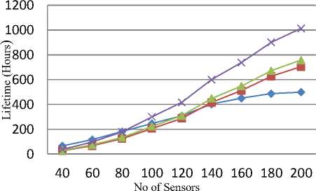
Fig. 1(a)

ALBPS

2-Level Heterogeneity

3-Level Heterogeneity

Multi-Level Heterogeneity

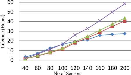
Fig. 1(b)

Fig. 1(a) & (b): The total network Lifetime for different number of sensors at 30 M adjustable sensing range and 50 Targets for Linear and Quadratic energy model (m=0.2 and a =3 for 2-level; a =1.5, в =3, m=0.5 and m0=0.4 for 3-level)

We now discuss the effect of sensing range on the lifetime of sensor networks for the given number of sensors. The sensors are categorized based on the parametric values as given in Table I (case I and case II for 2-level and 3-level). We have deployed 200 number of sensors out of which 160 are normal and 40 advanced nodes for 2-level heterogeneity. An advance node has 3 times more energy than a normal node. In case of three-level heterogeneity, there are 40 super nodes equipped with 3 times more energy than the normal nodes and 60 advanced nodes deployed with 1.5 times more energy than normal nodes.

— ♦ — ALBPS

—*— 3-Level Heterogeneity

— ■ — 2-Level Heterogeneity

Multi-Level Heterogeneity

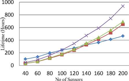
Fig. 2(a)

— ♦ — ALBPS

▲ 3-Level Heterogeneity

■ 2-Level Heterogeneity

Multi-Level Heterogeneity

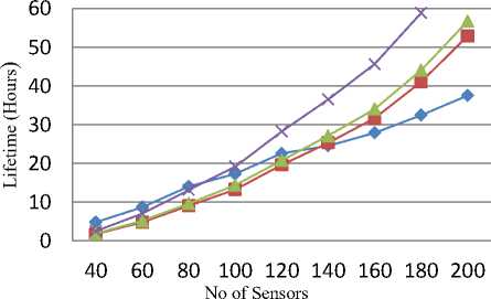
Fig. 2(b)

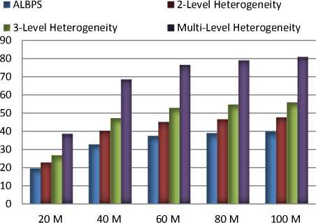
Fig. 2(a) & (b): The total network Lifetime for different number of sensors at 60 M adjustable sensing range and 50 Targets for Linear and Quadratic energy model (m=0.2 and a =3 for 2-level; a =1.5, β =3, m=0.5 and m0=0.4 for 3-level)

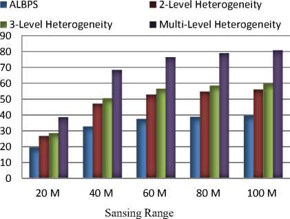
Fig. 3: Network lifetime for different adjustable sensing range values at 200 number of sensors, 50 Targets for quadratic energy model (m=0.2 and a =3 for 2-level; a =1.5, β =3, m=0.5 and m0=0.4 for 3-level)

For case II, in 2-level heterogeneity, there are 20 advanced nodes with 5 times more energy than normal nodes. In 3-level heterogeneity, there are 20 super nodes deployed with 3 times more energy than normal nodes and 20 advance nodes deployed with 1 times more energy than the normal nodes. In multi-level heterogeneity, all the nodes have different level of energy within the interval of [0.5, 2].

Sensing range

Fig. 4: Network lifetime for different adjustable sensing range values at 200 number of sensors, 50 Targets for quadratic energy model (m=0.1 and a =5 for 2-level; a =1, β =3, m=0.2 and m0=0.5 for 3-level)

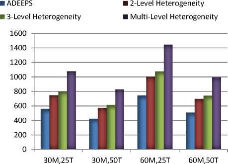
Now, we discuss the effect of maximum sensing range alone with number of targets on the lifetime of sensor network for 200 numbers of sensors which have been categorized above among different types of nodes based on the level of heterogeneity. We consider 25 and 50 targets randomly distributed and we vary sensing range 30 M and 60 M using linear and quadratic energy models.

■ 2-Level Heterogeneity

■ ALBPS

■ 3-Level Heterogeneity

■ Multi-Level Heterogeneity

■ ALBPS

• ■ 2-Level Heterogeneity

• ■ 3-Level Heterogeneity

  ■ Multi-Level Heterogeneity

  

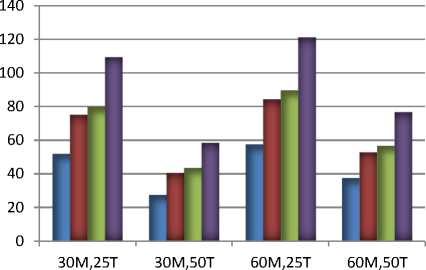
  Fig. 5(b)

  
  

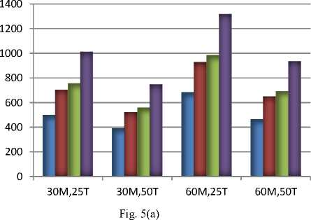
Fig. 5(a) & (b): Network lifetime for different adjustable sensing range and target values at 200 number of sensors for linear and quadratic energy models (m=0.2 and a =3 for 2-level; a =1.5, β =3, m=0.5 and m0=0.4 for 3-level)

• ■    ALBPS

• ■    2-Level Heterogeneity

decreases for the given sensing range. In this case also as the level of heterogeneity increases, the lifetime increases. We obtain similar results for case II as shown in Figs. 6(a) and (b). The results are consistent with the previous results because the network lifetime increases with the decrease in the number of targets.

г 3-Level Heterogeneity

Fig. 7(a)

■ Multi-Level Heterogeneity

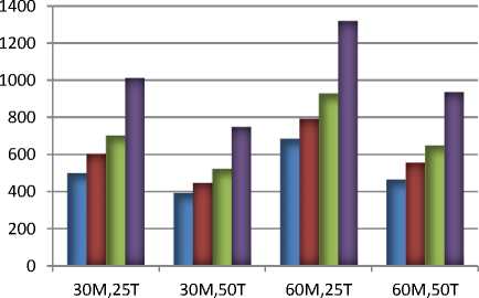
Fig. 6(a)

■ ALBPS                          ■ 2-Level Heterogeneity

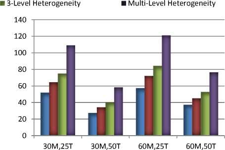
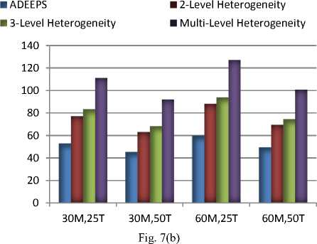
Fig. 7(a) & (b): Network lifetime for different adjustable sensing range and target values at 200 number of sensors for Linear and Quadratic energy model (m=0.2 and a =3 for 2-level; a =1.5, β =3, m=0.5 and m0=0.4 for 3-level)

Fig. 6(b)

Fig. 6(a) & (b): Network lifetime for different adjustable sensing range and target values at 200 number of sensors for Linear and Quadratic energy model (m=0.1 and a =5 for 2-level; a =1, β =3, m=0.2 and m0=0.5 for 3-level)

We observe from Figs. 5(a) and (b) that increasing the number of targets, the lifetime of a sensor network

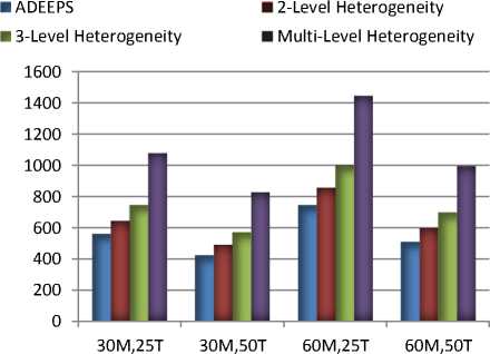
Fig. 8(a)

■ ADEEPS

■ 3-Level Heterogeneity

■ 2-Level Heterogeneity

■ Multi-Level Heterogeneity

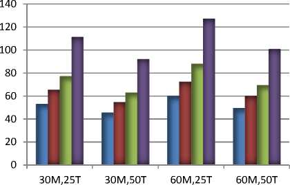
Fig.8(b)

Fig. 8(a) &( b): Network lifetime for different adjustable sensing range and target values at 200 number of sensors for Linear and Quadratic energy model (m=0.1 and a =5 for 2-level; a =1, β =3, m=0.2 and m0=0.5 for 3-level)

— ■ — 2-Level Heterogeneity

— ♦ — ADEEPS

—*— 3-Level Heterogeneity

Multi-Level Heterogeneity

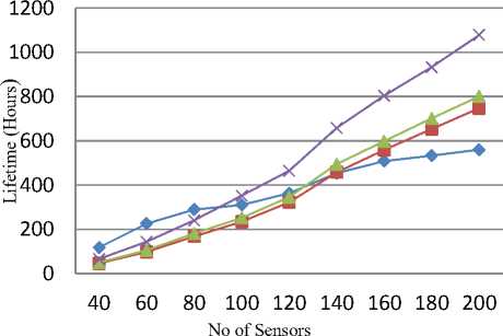
Fig. 9(a)

• ADEEPS

■ 2-Level Heterogeneity

—*— 3-Level Heterogeneity

Multi-Level Heterogeneity

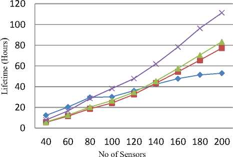
Fig. 9(b)

Fig. 9(a) & (b): The total network Lifetime for different number of sensors at 30 M adjustable sensing range and 25 Targets for Linear and Quadratic energy model (m=0.2 and a =3 for 2-level; a =1.5, β =3, m=0.5 and m0=0.4 for 3-level)

For ADEEPS with heterogeneity, we have obtained similar results as obtained for ALBPS with heterogeneity. The corresponding results are shown in Figs. 7(a)-(b), 8(a)-(b), and 9(a)-(b). The protocols ALBPS and ADEEPS [4] are for homogeneous networks. Therefore, it is not justifiable to compare their performance with that of the proposed ones as they are meant for heterogeneous networks. However, for the sake of reference, their simulation results have also been given along with that of the proposed ones.

V. Conclusion

In this paper, we have discussed two new protocols by incorporating different levels of heterogeneity in ALPBS and ADEEPS. The outcome of the paper can be summarized as follows. The proposed protocols perform better than their homogeneous counterpart for all levels of heterogeneity. As the level of heterogeneity increases, the lifetime also increases. For the given number of targets and sensing ranges, the network lifetime increases with the number of sensors. When the number of targets is increased, the network lifetime decreases as more targets are monitored by the fixed number of sensors.