Performance Evaluation of Image Segmentation Method based on Doubly Truncated Generalized Laplace Mixture Model and Hierarchical Clustering

Image segmentation aims at identifying the regions of interest in an image or annotating the data of an image. It is the process to classify an image into several clusters according to the feature of image. Image segmentation techniques are based on some pixel or region similarity measures in relation to their local neighborhood. Segmentation techniques are broadly classified as region based, edge based, threshold based and model based [14]. Among these model based segmentation algorithms are found to be efficient compared to other [5]. In model based, entire image is viewed as a collection of image regions and each image region is characterized by a probability distribution function of pixels.

The pixel intensity is considered as a feature component of the image. The pixel intensities in image may be meso kurtic, platy kurtic, lepto kurtic, symmetric and asymmetric. The efficiency of segmentation algorithm depends on probability distribution followed by the pixels in an image.

Much work has been reported considering the pixel intensities follow a Gaussian distribution and variates of finite GMM. Yunjie Chen et al[6] analyzed Gaussian Mixture Model based on Non Local Information for brain MR images segmentation. Legendre polynomials were used to fit and merged to the EM framework and non local information was also used to preserve the geometrical edges information. Karim Kalti et al[7] analyzed an image segmentation method based on Gaussian Mixture model and modified FCM Algorithm. The classification was made on the basis of adaptive distance which privileged the one or the other features according to the spatial position of the pixel in the image. Zhaoxia Fu et al [8] proposed an image segmentation method which used Gaussian Mixture Models to model the original image and transforms the segmentation problem into maximum likelihood parameter estimation by expectation-maximization(EM algorithm) and classify the pixels in image. The application of GMM is accurate and successful for all types of data except lepto kurtic. To overcome this drawback generalization of Gaussian mixture models with respect to kurtosis is considered. Laplace probability model serves as a alternate to Gaussian distribution with respect to platy kurtic, lepto kurtic and asymmetric data. Srinivasa Rao et al[9] generalized the laplace distribution as generalized Laplace distribution. Jyothirmayi et al[10] later developed and analyzed the generalized Laplace mixture model(GLMM) for image segmentation. In these algorithms the range of pixel intensities was assumed as {-∞,∞}.

The developed model was integrated with hierarchical clustering method and used for image segmentation of images which are having platykurtic and lepto kurtic nature. Hierarchical clustering and moment method of estimation was used for initialization of parameters. As an extension to the previous works, within the current work an attempt is made to extend the GLMM as Doubly Truncated GLMM (DTGLMM) by truncating the range of pixel intensity values within a specified range. Performance evaluation of the developed model has been carried out by means of analysis of various different categories of images as case studies.

• II.    Proposed Work

In this paper an algorithm DTGLMM-H has been proposed for image segmentation. It is assumed that the whole image is collection of image regions in which the pixel intensity of each region follows a generalized laplace distribution. The parameters mean, variance of DTGLMM are estimated through EM algorithm. Initialization of the parameters is obtained by hierarchical clustering. Image analysis with the developed algorithm is performed on five images from Berkeley image data set and compared with existing algorithms available in the literature

• A.    Doubly Truncated Generalized Laplace Distribution

An image is considered as a collection of image regions for segmentation algorithms. Each image is quantized by pixel intensities. The pixel intensity z=f(x,y) is a random variable for any given point in image region.

The pixel intensities within the region are assumed to have an infinite range. But in any image the pixel intensity lie between two values. Assuming that the pixel intensity lie between ‘a’ and ‘b’, the probability density function of the pixel intensity is given by

f ( X , µ , О-²)

(г2+(I - µ) )е|| у2 ∑к=0

where a< X0

This can also be represented as

/( X , µ , а² )

(г2+( * -к) )е|| var(x) = var( ; ∑i=l Хi)=

∑ =  (2)(     )2’qa4 [                  ( -*),y [(,+l), ( ? )]]

" w к(-1) Qy[(q+3), (   )] +Y[(q+1), (   )] +Y[(q+3), ()]

∑k=0(к) Г2 ( ,-k)[ Y [(2k+l), (   )] "Y[(2k+l),()]]

• B.    Estimation of the Model Parameters By EM Algorithm

To estimate the model parameters, EM algorithm is utilized by maximizing the expected likelihood function. It is assumed that the intensity of pixel in image region follows a new Laplace distribution and whole image is characterized with a finite mixture of new generalized Laplace distributions. To get accurate result doubly truncated generalized Laplace distribution is well suited where range of pixel intensities is assumed to be finite. Its probability distribution function is given in equation 2.

The likelihood function of observations x1,x2….xn is

^{α = ∑    Т} i (x, θ ¹ ) = ∑    [ к α( ? ,θ) ; ]

∑ α (xs,θ )

For updating the parameter µi, i=1,2,..k

Consider the derivative of Q( 6 ; 9^l ) with respect to µ i , and equate to 0

_Q( e ; e^l ) =E[log L(( e ; e^l ) ]          (11)

µ1 Q( 6; 01)=0

This implies

L( e )= ∏ S-1P (x, 6^l )

(i.e) L( e )=∏ S = 1 (∑i=l «t ft (x, Hi , Oi²))       (5)

Log L( 9)= ∑S=1log(∑ ^a-ifi (x, Hi , о² ))

where

∂∂µі⎢⎢∑∑Т(x, )

(_r2+ ⁽ X - µ ) ) e_{|   |}

2 a ∑    ( к )⁽ r-k ⁾(∫ A x^2ke || dx )

+ log(αi1)⎥=0

0 ={ ц , O"² , a_t ;i=1,2,..k}

Log ∑ s=i log [(

(^{( µ )})      ^{|       |}

2o ^∑L„ (£)^{(  )}(∫ A X^2k6 || ax

) )]

This implies

к N

E Step: In the E Step the expectation value of log L( 9 ) with respect to initial parameter 9° is

∂ ^∂ µ і⎢ ^⎢∑∑Т ‘ (x,⁶‘)⎢ ^⎢ tog

i=l s=l

[((r- ⁺

(x

-

µ , )

))]

Q( e ; e° )= E_e» [log L ( e )]              (7)

P( x_s ,θ¹ )= ∑i=l ^αi¹fi(x, θ¹)

Log L( e )= ∑^=1log(∑b=i ^α i¹fi(x, θ¹))      (8)

The conditional probability of x s belonging to region k is

-1/2|  - µ i |-log(a, )

-log(∑ (rk ) r2()∫x2ke k=0            а-Ц

=0

^| x ^| dx )⎥ + log( α t¹)

This implies

Tk(x, θ1     ^αk^lfk(^xs,θ)       α k^lfk ( ^xs ,θ)

k ,            (Xs,θ )    = ∑ tl αi'fi(Xs,θ)

Q( e ; 0° )= ∑b=i ∑ ^=1 Т i (x, θ)(log f i (x, θ¹) +log αi¹

N

∑Т , (x, θ ¹ ) [( ⁽

S = 1

x

-

^µ ' ⁾ )[

[-2 о ² ]

r2^2+(x

-

µ , )

Where

f i (x, θ ¹ ) = (

(       ( µ ) ) |       |

2o ^∑    ( к )⁽ r-k ⁾(∫ i °p x^e^{- | |})

)

+ ^σ i   ]]=0

|x - μi^|

^∑ ^=1 Т i (x, θ¹)       μ| ^{- ∑} S = 1Т i (x, θ¹) ^[-(µ)] _{2 =0}

^σ | ^μ |                                             (µ_i)

M Step: To get estimation of parameters, maximize Q( 0 ; 0^l ) such that ∑ α i =1.

Using Lagrange type function and maximizing

where

T i ( x s , θ^l ) =

α i^l * ¹ f i ( x s , θ^l )

∑ _i ^k 1 ^αi ^l+1 f i ( x s , θ^l )

̂ =   ∑ ^=1 Тi(x, θ¹)            (10)

αi for (l+1)th iteration is

For For updating σ i² differentiate Q ( θ;θ¹) w.r.t σi² аnd equаte to 0

Q ( θ;θ¹)=0

∂

∂ ^l2

к N

∑∑Т , (x , e^l )

i=l s=l

log ⎢ ^⎢⎡ ⎜ ^⎛

( _T2 + ⁽ 1 - µ ) -)e |    |

⎤

This implies

к N

∂ ^∂_?⎢^⎢∑∑Т(x ,O')⎢^⎢ log

i=l s=l

[((  +(x

-

=0

⎢2 <1 ^∑к) _r2(   )(_∫

b-jl

'a-ц X

2kg- ^| x ^| dx )

⎠⎦

+ log( α i¹)

=0

µ )

»i2

))] -| X_S -µ |-log( at ) -log(∑ ( \ ) r² (  ) ₍∫ x^2ke || dx )

¹                     k=O               a-p

+ log(αi1)

This implies

N

∑

(x -µ)

( r²a_t² +(x ^-µ) ) ad

| x_s -µ _|

|₂ ad I

2 ad

^{∑ T}k=» ⁽I^{) r}l ⁽2 ) [( - - µ _{) ․} - - µ _.^e" |   | -( - µ _{) .} - - µ _.^e" |   |

∑ l„ ( к )   ( r-_k ) (_∫ Л x^2ke || dx

Т (x,θ1)=0

where

Т i (x ,θ*)=

α i     fi(x , θ J )

∑ ^α .1+1 f i (x ,θ*)

solving the equations 13 and 15 we can get the final estimates of the parameters μ i and σ 2 .

• C.    Initialization of the Parameters By Hierarchical clustering algorithm

  The parameter α_i and the model parameters µ аnd σj² have to be initialized for EM algorithm. The value for α_i= 1/k where k is the number of image regions. The model parameters are obtained from hierarchical clustering (S.C. Johnson (1967)) and moment method of estimation. The truncation points a and b are estimated with minimum and maximum values of pixel intensities of the image. The shape parameter r can be estimated by sample kurtosis using the following equation

The mean of the distribution is

^β 2 ⁼

∑^r k 0 (_k^r) r^{2(r k)}∑⁴ q 0 (⁴_q)(μ-μ 1 ¹)^{4 q}σ^q

(-1)^{2k q}γ[(2k+q+ 1),-( ^a- _σ ^μ )]+ γ[(2k+q+1),( ^b- σ ^μ )]

^{∑ r} k 0 (_k^r) r^2(r k) ∑ 4 _{q 0}(²_q)(μ-μ₁¹)^{2 q}σ^q

(-1)^{2k q}γ[(2k+q+ 1),-( ^a- _σ ^μ )]+ γ[(2k+q+ 1), ( ^b- _σ ^μ )]

∑ ^r k 0 ( _k ^r ) r^{2 ( r k )} γ [( 2k + 1 ),-( ^a _σ ^μ )] + γ [( 2k + 1 ),( ^b _σ ^μ )]

x̅= μ +

∑ ^rk 0 (_k^r) r ^{2 ( r k )}[γ[(2k⁺ 2),( ^b σ ^μ )] γ[(2k ⁺ 2), ( ^a _σ ^μ )]

∑ ^rk 0 (_k^r) r ^{2 ( r k )}[γ[(2k+1),( ^b _σ ^μ )] γ[(2k +1), ( ^a _σ ^μ )]

and σ ² =

∑q-0(^ )(n-ni) -%.

⁽-¹⁾ q_Y[(q+l), (    ) ] ⁺⁽-^{1 )} q_Y[(q+3 ), (   )]

+Y [(q+i), ( ^ )] +Y[(q+3), ( ^ )]

^∑ Lo ⁽ r ⁾ r^{2 (} r-k⁾[ γ [(2k+l), ( σ ^μ )] γ [(2k+l),( - _σ μ _)]]

Solving equations 16, 17 and 18 simultaneously by Newton Raphson Method the parameters μ and σi2 are obtained. With these initial estimates final estimates are obtained through EM algorithm as illustrated in section B.

D. Segmentation Algorithm

Once the final estimates of parameters are obtained, next step is to segment the image by assigning the pixels to segments. This is achieved through the following segmentation algorithm.

Step 1: Attain the number of image segments using hierarchical clustering algorithm.

Step2: Obtain the initial estimates of model parameters using hierarchical clustering.

Step 3: Using the EM algorithm obtain the refined estimates of the model parameters α_i, μ_i, σ_i ² for i=1,2….k.

Step 4: Assign each pixel to corresponding j ^th region according to maximum likelihood of the segment L j . The pixel z_s is assigned to the j ^th segment for which L is maximum.

Table 1. Estimation of parameters for Image1

Estimated Values of the Parameters for Image1 Number of regions(K=3)
Parameters	Estimation of Initial Parameters By Hierarchical Clustering			Estimation of Final Parameters by EM Algorithm
	C1	C2	C3	C1	C2	C3
α i	0.33	0.33	0.33	0.136	0.985	0.150
μ i	102.72	244.9	148.3	251.9	198.3	261.1
σ i	10.79	6.90	15.29	13.37	51.31	40.74
a=0				b=255

L=mаx

(

⁽_r2+(µ) ) |      ^|

ь-ц

∑U(£) r2 ( r-k )(∫           | |dx )

)

III. Experimentation and Results

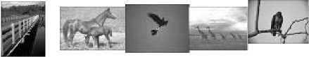
For experimentation five images randomly were taken from         Berkeley         image         dataset

( ds/BSDS300/html/dataset/. The pixel intensity values in image are chosen as feature of the image assuming that they follow generalized Laplace distribution. Image consists of K image regions and initial value of K is obtained by histogram of pixel intensities. The five images and their respective histograms are shown in figure1.

Image

Histogr am

Fig.1. Images and their Histograms.

The model parameters considered are α_i, μ_i and σ_i for i=1,2…K and are obtained by the method given in section 4. Final parameters for the five images have been derived using these initial parameters and updated equations in section 3 the final parameters and presented in t ables 1,2,3,4 and 5 .

Table 2. Estimation of parameters for Image2

Estimated Values of the Parameters for Image2 Number of regions(K=3)
Parameters	Estimation of Initial Parameters By Hierarchical Clustering			Estimation of Final Parameters by EM Algorithm
	C1	C2	C3	C1	C2	C3
α i	0.33	0.33	0.33	0.43	0.43	0.13
μ i	185.37	151.79	69.28	190.55	48.16	111.8
σ i	9.42	8.95	11.13	15.53	11.30	18.2
a=34			b=254

Table 3. Estimation of parameters for Image3

Estimated Values of the Parameters for Image3 Number of regions(K=3)
Paramete rs	Estimation of Initial Parameters By Hierarchical Clustering			Estimation of Final Parameters by EM Algorithm
	C1	C2	C3	C1	C2	C3
α i	0.33	0.33	0.33	0.352	-0.021	0.668
μ i	144.5	53.46	180.8	170.5	49.37	194.8
σ i	7.21	16.03	4.94	18.53	18.30	15.24
a=7				b=187

Table 4. Estimation of parameters for Image4

Estimated Values of the Parameters for Image4 Number of regions(K=3)
Parameters	Estimation of Initial Parameters By Hierarchical Clustering			Estimation of Final Parameters by EM Algorithm
	C1	C2	C3	C1	C2	C3
α i	0.33	0.33	0.33	0.7666	0.0018	0.2343
μ i	242	34.33	179.79	193.86	58.16	159.80
σ i	12.63	5.85	18.36	10.09	13.70	20.27
a=30				b=255

Table 5. Estimation of parameters for Image5

Estimated Values of the Parameters for Image5 Number of regions(K=3)
Parameters	Estimation of Initial Parameters By Hierarchical Clustering			Estimation of Final Parameters by EM Algorithm
	C1	C2	C3	C1	C2	C3
α i	0.33	0.33	0.33	-0.18	1.23	-0.04
μ i	110.91	190.53	51.08	24.05	116.42	72.04
σ i	14.39	14.82	18.62	10.53	14.30	13.26
a=5				b=231

20.18

(1+

271.4(1+

40.54

f(x,θ^l ) = ( X - 193.8)²

10.092

( X - 58.16) ²

13.7

(1+

)     _| х-193 ^. 5|

|     .09 |+

)      | х-58 ^. 15.1

е|     .7 |+

( X - 159.80) ² 20.27

)     | х-159 ^. 80 |

|                                .                                |

The estimated probability density function of the pixel intensities of the image5 is

Substituting the final estimates of the model parameters the probability density function of the pixel intensities in each image are estimated.

The estimated probability density function of the pixel intensities of the image1 is

21.06

1 28.60

(1+

(1+

f(x,θ^l ) =

( X - 24.05) ²

10.532

( X - 116.42) ² 14.30²

) ;"|

) е"|

Х-24 ^. 05 I .

I 10.S3 |+

х-116 ^. 42 I .

I 18.30 |+

26.52

(1+

( X - 72.04)²

13.262

)

	f(x,θl ) =
1( X - 26.74 (1 +	251.93)2у 13.372    )
1   (1+(^ - 102.62 ( +	- 198.30)2у 51.312    )
1( X 81.48 ( 1 +	- 261.12)2\ 40.742    )

| Х-261 ^. 12 |

5   |         .         |

| х-198 ^. 30 |

5 |     .31  |+

| X—251 ^. 93 |

5|     .37  |+

Using the probability density function and segmentation algorithm, image segmentation is performed for following images. The original images and segmented images are shown in Figure 2.

The estimated probability density function of the pixel intensities of the image2 is

31.06

(1+

f(x,θ^l ) = ( X - 190.55)²

221.6(1+

15.532

( х - 48.16) ²

11.302

)     | х-190 ^. 55 |

|      .S3 |+

)     | Х-48 . 16 | е|     .зо |+

¹   (1+ ⁽   - 111.8) : )е ^| 18. # ^{. |}

36.4 ⁽¹⁺     18.2     ⁾

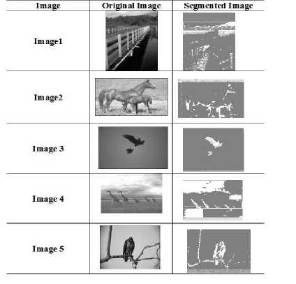
Fig.2. Original Image and Segmented Image

The estimated probability density function of the pixel intensities of the image3 is

37.06

(1+

f(x,θ^l ) = ( X - 170.55)²

¹ 36.6 ⁽

30.48

1+

18.532

( X - 49.37) ²

18.32

)     | Z-170 ^. 55 |

|      .S3 |+

)     _| Х-49 ^. 37 |

|     .30 |+

(1+

( X - 194.80) ² 15.24²

)     | Z-194 .8| е|         .         |

The estimated probability density function of the pixel intensities of the image4 is

IV. Performance Measures

Once the image segmentation has been performed, its performance has been measured by calculating the performance metrics like probabilistic rand index(PRI) given by Unnikrishnan R et al(2007), global consistency error(GCE) given BY Martin D. and et al and variation of information (VOI) given by Meila M(2005). The standard criteria for metrics is that PRI and GCE values must lie in range 0 to 1 while VOI can take value as big as possible. The performance metrics for image segmentation method based on doubly truncated generalized mixture model using hierarchical clustering

(DTGLMM-H) is shown in table 6 and compared with segmentation method based on GMM, GLMM using K-means (GLMM-K), GLMM using Hierarchical clustering (GLMM-H) and doubly truncated generalized mixture model using K-means algorithm (DTGLMM-K).

From table 6 it is observed that the proposed method satisfies the standard criteria for the performance measures PRI, GCE and VOI. The performance metrics are compared with GMM, GLMM-K, GLMM-H and DTGLMM-K and presented in Figure 3.

The image can also be reconstructed using the developed algorithm. Different quality metrics like image fidelity mean square error and image quality can be computed to study the performance of image quality. The metrics have been calculated and shown in Table7.

From Table 7 it can be seen that the proposed method DTGLMM-H has performed well when compared with other methods.

The original images and reconstructed images using developed segmentation algorithm are presented in figure 4.

Table 6. Performance Measures

Image	Method	Performance Measures
		PRI	GCE	VOI
Image1	GMM	0.94	0.72	2.84
	GLMM-K	0.98	0.73	5.31
	GLMM-H	0.99	0.68	2.25
	DTGLMM-K	0.99	0.11	0.83
	DTGLMM-H	0.9988	0.1150	0.8164
Image2	GMM	0.96	0.78	2.55
	GLMM-K	0.98	0.75	5.22
	GLMM-H	0.98	0.75	2.23
	DTGLMM-K	0.99	0.10	0.87
	DTGLMM-H	0.9975	0.1065	0.8749
Image3	GMM	0.97	0.77	2.32
	GLMM-K	0.97	0.71	5.20
	GLMM-H	0.98	0.75	1.48
	DTGLMM-K	0.99	0.10	0.85
	DTGLMM-H	0.9964	0.1029	0.8740
Image4	GMM	0.97	0.69	2.23
	GLMM-K	0.97	0.72	2.88
	GLMM-H	0.98	0.66	1.45
	DTGLMM-K	0.99	0.035	0.25
	DTGLMM-H	0.9980	0.0385	0.2702
Image5	GMM	0.96	0.77	2.12
	GLMM-K	0.98	0.75	2.34
	GLMM-H	0.97	0.73	2.02
	DTGLMM-K	0.99	0.10	0.72
	DTGLMM-H	0.9986	0.1027	0.7278

Table 7. Segmentation Quality Metrics

Image	Method	Image Quality Metrics
		Image Fidelity	Signal to Noise Ratio	Image Quality Index
Image1	GMM	0.99	0.24	1.0
	GLMM-H	0.99	0.24	0.988
	GLMM-K	0.99	0.419	0.988
	DTGLMM-K	.99	0.34	.99
	DTGLMM-H	0.99	0.38	0.9943
Image2	GMM	0.99	2.01	0.99
	GLMM-K	0.99	0.41	0.99
	GLMM-H	0.99	2.03	0.99
	DTGLMM-K	.99	3.34	.99
	DTGLMM-H	0.9985	4.21	0.9915
Image3	GMM	0.98	1.45	0.98
	GLMM-K	0.99	0.03	0.99
	GLMM-H	0.99	1.45	0.99
	DTGLMM-K	0.99	2.25	.98
	DTGLMM-H	0.9965	2.53	0.9836
Image4	GMM	.99	2.23	1.0
	GLMM-K	.98	4.4	.998
	GLMM-H	.99	2.69	1.0
	DTGLMM-K	1.0	4.5	.99
	DTGLMM-H	1.0	4.0	0.9998
Image5	GMM	.99	1.09	0.99
	GLMM-K	.99	2.67	.99
	GLMM-H	.99	1.13	.997
	DTGLMM-K	.99	3.77	.99
	DTGLMM-H	0.99	2.83	0.9925

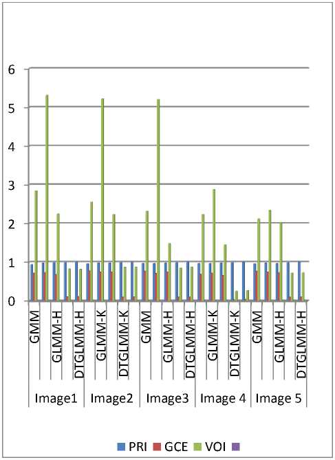
Fig.3. Comparison of Performance Metrics.

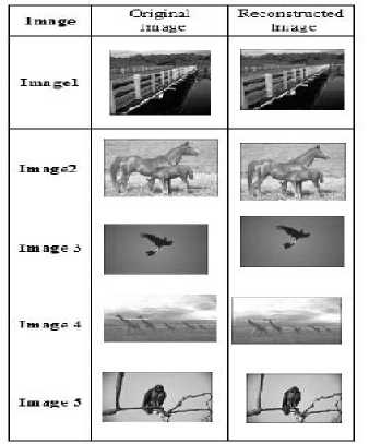
Fig.4. Original and Reconstructed Images

• V. Conclusion

This paper addresses the image segmentation method based on doubly truncated generalized Laplace distribution mixture model and hierarchical clustering. The feature vector associated with the image region is characterized by truncated generalized Laplace distribution which improves Laplace and generalized laplace distributions as limiting cases. The doubly truncated generalized laplace distribution includes a spectrum of probability models which may be meso kurtic, platy kurtic, lepto kurtic, symmetric and asymmetric. The effect of truncation on probability model has a significant influence since in reality the pixel intensities are having finite range. The model parameters are estimated by deriving updated equations of the scale and location parameters. The shape parameter is estimated using sample kurtosis. The initialization of parameter is carried using hierarchical clustering for initial segmentation for whole image and moment methods of estimation. The performance of the algorithm is analyzed through experimentation on randomly chosen five images from Berkeley data set. The performance measures such as PRI, GCE and VOI revealed that this algorithm perform better than the earlier algorithms. This may be due to the effect of truncation used for modeling feature vector. The hierarchical clustering algorithm used for initialization of parameters reduces the computational complexities and convergence of the EM algorithm. The proposed algorithm is much useful for analyzing images arising at several domains of applications. It is possible to extend this image segmentation method for color images considering a 3-dimensional feature vector which will be taken up elsewhere.